Экстракт Знаний

15 Spreadsheet Formulas Working Professionals Should Know!

14:42

15 Spreadsheet Formulas Working Professionals Should Know!

Jeff Su 24.08.2021 161 089 просмотров 4 968 лайков обн. 18.02.2026

Смотреть на YouTube

Поделиться Telegram VK Бот

Транскрипт Скачать .md

Анализ с AI

Описание видео

🔩 Grab my free Workspace Toolkit: https://academy.jeffsu.org/?utm_source=youtube&utm_medium=video&utm_campaign=065 👨🏻‍💻 Having worked in roles that required me to use Excel and Google Sheets extensively over the past 7 years, I thought it might be good to share 15 Google Sheets Formulas that all Working Professionals Should Know! Whether you're a beginner who have never come across Google Sheets functions, or a power user who feel comfortable combining multiple Google Sheets formulas, I hope there's something for you in this Google Sheets / Excel formula video! For simple formulas that most people use such as VLOOKUP, there are things you want to watch out for, for example when to use "TRUE" vs. when to use "FALSE." We also cover more advanced formulas such as IMPORTRANGE, ARRAYFORMULA, CONCATENATE, and combined functions such as =IF(SEARCH()) If you're a fresh graduate who just landed a first full-time job, or a working professional who has been working for 1-5 years, you probably will come across situations where you would need to use some (if not all) of the formulas mentioned in this video, whether you work with Microsoft Excel or Google Sheets, so why not give yourself a head start by practicing today? 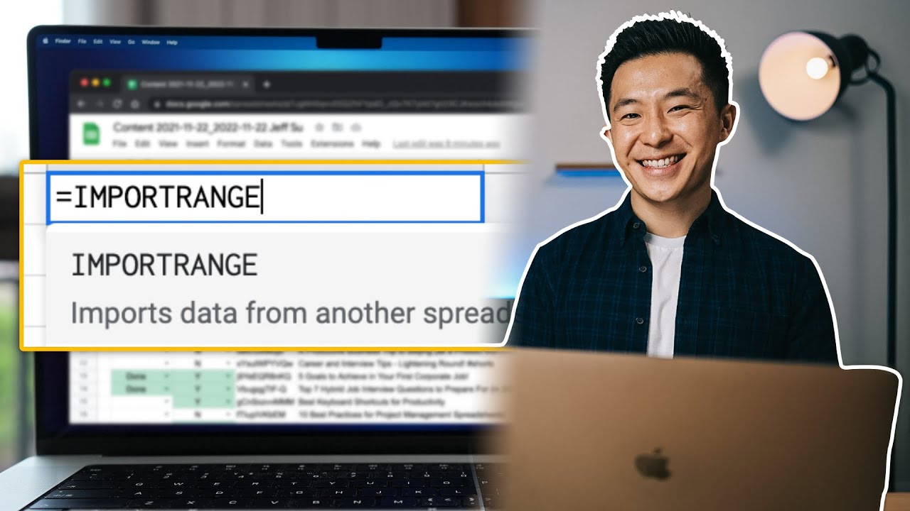😉 TIMESTAMPS 00:00 DETECTLANGUAGE 00:46 VLOOKUP mistakes 01:25 Wildcard Asterisk Character 01:50 TODAY 02:15 IMPORTRANGE 03:45 COUNTIF 04:08 COUNTA 04:48 SPLIT 05:43 LEFT 05:55 RIGHT 07:02 ISEMAIL and SUBSTITUTE 08:06 ISURL 08:31 ARRAYFORMULA 09:10 CONCATENATE 10:11 & 10:37 IF and SEARCH 11:49 IFERROR 12:22 SUMIF 13:45 TRIM, UPPER, LOWER, and PROPER RESOURCES I MENTION IN THE VIDEO 📧 Subscribe to my Productivity newsletter - https://www.jeffsu.org/productivity-ping/ MY FAVORITE GEAR 🎥 My YouTube Gear - https://geni.us/youtube-gear 🎒 What's In My Bag - https://geni.us/mybag 💻 What's On My Desk - https://geni.us/mydesk 🛩 What I Travel With - https://geni.us/mytravel MY FAVORITE SOFTWARE ✍️ Skillshare - https://geni.us/skillshare-jeff 🎨 Canva - https://partner.canva.com/jeffsu BE MY FRIEND: 📧 Subscribe to my Productivity newsletter - https://www.jeffsu.org/productivity-ping/ 📸 Instagram - https://instagram.com/j.sushie 🤝 LinkedIn - https://www.linkedin.com/in/jsu05/ 👋🏻 Clubhouse - https://www.joinclubhouse.com/@jsushie 👨🏻‍💻 WHO AM I: I'm Jeff, a full time Product Marketer. In my spare time I like to tinker with tools and create systems that help me get things done faster - or as one of my friends puts it: "Get better at being lazy" 😏 If you'd like to talk, I'd love to hear from you. Messaging me on Instagram (@j.sushie) directly will be the quickest way to get a response! PS: Some of the links in this description are affiliate links I get a kickback from 😇 Disclaimer: My opinions are my own and may not reflect that of my employer #formulas #functions #googlesheets

Оглавление (19 сегментов)

0:00 DETECTLANGUAGE 143 сл.
0:46 VLOOKUP mistakes 123 сл.
1:25 Wildcard Asterisk Character 59 сл.
1:50 TODAY 76 сл.
2:15 IMPORTRANGE 240 сл.
3:45 COUNTIF 70 сл.
4:08 COUNTA 117 сл.
4:48 SPLIT 161 сл.
5:43 LEFT 30 сл.
5:55 RIGHT 222 сл.
7:02 ISEMAIL and SUBSTITUTE 175 сл.
8:06 ISURL 79 сл.
8:31 ARRAYFORMULA 111 сл.
9:10 CONCATENATE 168 сл.
10:11 & 70 сл.
10:37 IF and SEARCH 206 сл.
11:49 IFERROR 94 сл.
12:22 SUMIF 242 сл.
13:45 TRIM, UPPER, LOWER, and PROPER 153 сл.

DETECTLANGUAGE

so if you saw characters in another language on google sheets what would you do well first you can use the detect language formula to first identify the language code then you can use the google translate formula to find out that jeff is simply the sweetest and he appreciates his audience all very much let's get started hi friends welcome back to the channel if you're new here my name is jeff and i'll admit that google translate formula is definitely not necessary for working professionals to know but you gotta admit it's pretty freaking cool in this video i share 15 or so google sheets formulas and functions that i've used the most over the past seven years as a working professional first as a management consultant and now is a product marketer at a fang tech company diving right into

VLOOKUP mistakes

vlookup so this is a formula a lot of us have been using for a while now it's a very basic one but there are two things i want to mention here a lot of people type in true for the fourth field here but this could sometimes lead to errors because true tells google sheets to find the closest match for example i want to find the phone model that billy gates bought which is the model s but now it returns model 3 which is what bill gates bought so if i change to true to false like so now the correct phone model s is shown because false tells google sheets to find the exact match second it can be

Wildcard Asterisk Character

very handy to use the wildcard asterix character with the vlookup formula for example if you know someone's name begins with ti you can simply write vlookup quotation ti asterix uh quotation marks again comma select the range three columns over and false as i just mentioned and find that timmy cookie has purchased the model x next if

TODAY

you see up here i have a days until launch field whereby subtract today's date from the product launch date now obviously the launch date itself never changes but i have the today formula here that updates today's date automatically it's just a handy little feature that i use all the time at work next up import range for those of you who don't know what this is you're simply making an exact copy of a

IMPORTRANGE

tab from the same file or a completely separate google sheets file the beauty of this is when the original file updates your import range copy updates as well for example i have a bi-weekly productivity newsletter i'll link this down below if you want to sign up and i always ask for feedback via google forms and google forms outputs all this data in real time in a google sheets format and i can import this raw data into a completely separate tab by doing this equals import range quotation marks i copy the link of the raw data tab and then close quotation marks comma quotation marks again the label or the tab name down here explanation mark and the range i want to import for example range a1 all the way through i don't know d a thousand let's say a1 colon d1000 and then quotation marks and close bracket enter uh if this is the first time you're doing this you might need to like click and allow the connection but after that you should see the data imported over just like this and you do this because you might want to change the formatting of the data or manipulate the data in some way by performing calculations and you don't want to mess with and potentially mess up the raw data and now that i've formatted the data i can perform some symbol calculations for

COUNTIF

example if i want to find the number of people who gave me five out of five for my newsletter i can simply use the count if formula here highlight the range for the points and choose the criteria i want to count for in this case five close bracket and now i know 13 people gave me five out of five and now i want to find the number

COUNTA

of people who gave me feedback and i can do this by using the count a formula and i can select any of the first three columns because it's only counting the number of values i selected and now i can see there are 32 people who gave me feedback in total and from percentage standpoint divide 13 by 32 and wow only 40. 6 percent of you gave me five out of five you ungrateful but it's okay i'm a nice guy i'll let this one go for now next up if i wanted to separate the date and time in the timestamp column here into two separate columns i can use the split formula like

SPLIT

this choose a cell i want to split and choose the delimiter is just a fancy way of calling like a space or a comma or a period there's a space between these two values here so i'm choosing space and this automatically splits the date and time into two separate columns this works for things like commas as well for example hello there general kenobi bonus points if you get this reference uh split this put the comma within the quotation marks close a bracket and there you go back to the real example now at the date and time in two separate columns i can drag this all the way down press command d or control d on windows to apply the formula to all the rows now in a more real-life situation let's say i want to just separate out the month for example 4 april 5 may i would simply use the left formula and pull out

LEFT

one character from the left like so and again drag this all the way down command d and i've separated all the months by itself similarly for years let's say

RIGHT

this newsletter span across different years i can simply use the right formula and pull out the four rightmost characters in a given cell like so and i drag all those way down now i can dive into the performance for specific months and see those numbers in aggregate before we leave in pro range a pro tip i like to share is to always include the url of the raw data up top so you can easily refer to it and a brightly colored cell that reminds you and your teammates that there is an import range formula below so you don't want to like edit it by mistake for example by typing something here the entire table breaks don't do that by the way and i ask a lot of people this because i'm a nerd uh what is a formula that you use a lot but is very uncommon it could be a combination of different formulas or it could be one that no one has really heard of let me know down below now moving on to the next tab and let's say you receive some data from a colleague who shall we say isn't the most detail oriented and you want to double check his or her work before you do anything else first in order to

ISEMAIL and SUBSTITUTE

determine the emails here are indeed correctly formatted you want to use the is email function and select the cell you want to check and then drag this down uh true equals it's correct false means it's wrong upon further inspection for these three you'll see that there's no add symbol before gmail. com an easy fix for this is to use the substitute formula choose a cell you want to like quickly edit type out the incorrect portion of it in which case is gmail. com and then type in the correct version which is at gmail. com quotation marks close bracket and now you have perry gmail. com and because these three are the incorrect ones you can simply drag this down press command d press command c to copy and paste without formatting by pressing command shift v on mac and ctrl shift v on windows i think and this should all update to true and now you can delete the formula down here then if there are web pages here if

ISURL

you want to check whether these are formatted correctly you can use the is url function works exactly the same way uh select the cell you want to check drag all the way down false means there's something wrong with it true means it's fine for the two false ones you'll notice actually there is no dot before the com and now you can use the substitute like formula again to make those edits now pro tip in real

ARRAYFORMULA

life you're probably working with a lot more data for example there are 88 emails here and you want to check all of them at once right you can use the array formula function and have the is email embedded within and simply check choose the entire range you want to check as opposed to just one cell and if i close bracket here press enter this returns everything at once uh saving me the time to have to drag to the right and drag down and what not and of course array formula works with most of the other google sheets functions as well okay back to the marketing campaign

CONCATENATE

so you usually give clients a uid or unique id for them to use to log in or identify themselves and a very easy way to assign uids on in bulk is use the concatenate formula that combines values from different cells together for example if i want to use their location comma and their phone number to give them a uid i press enter and now there's a unique string assigned to this one client wendy but obviously this is not very privacy friendly so what i would do instead is simply add a write function which i went through just now and assign perhaps the last four digits of wendy's phone number by pressing four here and then i add another bracket to close this out and now she has a unique id that is both unique and privacy friendly all i need to do now is drag this down and voila quick and easy alternatively you want to make this slightly easier what you can

&

do instead is actually use a combination of left and right formulas for example i take the left most two characters from the first name of the client uh choose two and then use the and sign here and then follow that with the right formula and again choose the last four digits of their phone number and this also works as a way to assign uids on mass next

IF and SEARCH

formula a tiny bit more complicated but extremely useful and that is combining the if and search functions together for example if you look at the marketing channels here you notice there are organic channels and pay channels and i want to separate them out in a channel type column here first i'll use the search function and use the asterisk wildcard character again because i don't care what comes before the word organic and i use it after because i don't care what comes after quotation marks and choose the cell i want to reference like that and it returns one because it has found the organic word within this cell now because the number one by itself is meaningless i want to add the if formula on top of this to show me that if it finds the word organic please return the word organic like so if not leave it blank now it shows organic notice what happens when i drag this down and we see a few errors here this is to be expected now i can leave the errors as is because i know if there's an error it just means paid but i can take this a step further and

IFERROR

use the if error formula and if there is an error please return the word paid like so press enter and i drag i copy this paste it here and drag this all the way down and here is a very clean column that shows me exactly which challenges are organic and which ones are paid and while this three formula combination may look a bit scary at first the trick is to start with the formula inside in this case like search then work your way out and now that we've identified the

SUMIF

organic and paid channels i want to know how much each channel is contributing to sales so i use the sum if function here choose the channel type range press function f4 to lock this range in place choose the organic channel i can either type it out in quotation marks or simply choose the cell here comma again and choose the range i want to sum up and again press function f4 to lock this in place close out the formula press enter and boom uh organic channels contribute 4714 to my overall campaign now because i have so intelligently locked the ranges in place i can simply uh drag this down by pressing command d and this will repeat the process for the paid channel i can get a quick sense check here to make sure my calculations are correct if i highlight these two i see the sum is five hundred and ten dollars and if i sum up these i see it's ten thousand five hundred ten dollars so my calculations are probably correct i wanna quickly point out that yes i could have done that manually using the sum formula or the addition sign but that's prone to human error and in real life you're probably working with a lot more data and by using formulas like some if correctly it's physically impossible for you to make a mistake so why not and the last tab here

TRIM, UPPER, LOWER, and PROPER

consists of four very common formatting formulas i use whenever i receive raw data for example i get rid of needless spaces by using the trim function like so the upper formula just changes everything to case and a surprise lower means changing everything to lower case and there are times where you need to do this before inputting the data in a database and proper is simply changing the first character of every word to uh capitalized i'm not exactly embarrassed to admit this but i am a nerd when it comes to spreadsheets because i need everything to be structured and accurate right so please let me know if there are any cool formulas that you use that i could perhaps apply myself feel free to check out this video on some overall google sheets tips and tricks see you all next week and in the meantime have a great one

Ещё от Jeff Su

Write an Incredible Resume: 5 Golden Rules!

Jeff Su | 10.02.2021 | 9 сегм. | 4 283 593

AI Agents, Clearly Explained

Jeff Su | 08.04.2025 | 6 сегм. | 3 761 430

Master the Perfect ChatGPT Prompt Formula (in just 8 minutes)!

Jeff Su | 01.08.2023 | 10 сегм. | 3 433 903

Google’s AI Course for Beginners (in 10 minutes)!

Jeff Su | 14.11.2023 | 6 сегм. | 3 198 491

99% of Beginners Don't Know the Basics of AI

Jeff Su | 03.09.2024 | 7 сегм. | 2 861 212

5 Resume Mistakes You MUST Avoid (with real examples)!

Jeff Su | 23.08.2022 | 6 сегм. | 2 591 575

Ctrl+V

Экстракт Знаний в Telegram

Транскрипты, идеи, методички — всё самое полезное из лучших YouTube-каналов.

Подписаться