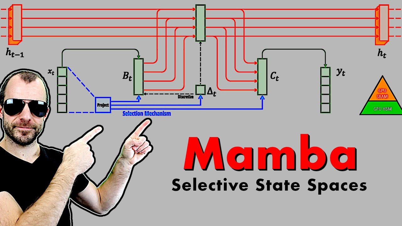
Mamba: Linear-Time Sequence Modeling with Selective State Spaces (Paper Explained)

hello today we're going to look at Muma linear time sequence modeling with Selective State Spaces by Albert goo and Tre da I know I'm a bit late on this paper uh but I still thought I'd give it a look and excuse the lack of face cam today I know it's a tragic loss to not see my face while doing these reviews I hope you can survive it uh so Mamba has been really big uh hailed as a poten itial competitor to Transformers uh has better scaling property scales to really long sequences and so on and yeah I wanted to know what it is and essentially two things like how does it differ from all the other stuff

that exists today uh because there there's so much stuff for example there are so there are the Transformers and those obviously have their advantages and problems then there are on are like rnns like recurrent neural networks and then there are these you know State space models like S4 or something like this and there's always interesting tradeoffs between all of those notably um what will see is in the Transformer you have if you have a sequence of stuff you have attention that's essentially anything can look at anything else and if you have causal attention if I look at this input I'm able to selectively look back at another input and sort of use that in the computation uh of the next layer here okay so a Transformer is able to dynamically and selectively look at individual elements of the past and address each one individually but obviously you have a problem with that so the problem with that is that you have like L squar when L is the sequence length l squ computations or n SL or n l squ uh memory requirements in order to do this rnns on the other hand if you have a sequence there they if you consider this um this particular input and you want to compute the next layer you can only look back one time step in fact you can't even look at the last input you what you will do is from each input you will compute a hidden state so there's going to be some sort of a box here and you will update the box and then the next thing will come and it will update the box and so on so you're only allowed to look at the last box and the current input if you want to decide what the next box here should be and from the box you obviously then compute the outputs so this is super restrictive in that you can only ever look at the last hidden State and the current input in order to compute the current output and the next hidden state but also this essentially scales to infinite lengths because it instead of having you know this much requirement of memory it only has actually it doesn't even it has L computation so you compute as many elements as you have right uh but then it the memory requirements are really they're really all of One they're really only how big is the hidden State and how big are the inputs and outputs now if you want to do back propop here that's when it becomes you know a bit more iffy then you will actually have to remember the whole sequence of intermediate values in order to back propagate so ornin use a thing that's called back propop through time and I know this is super old school and before most of you were born but again consider the thing where you compute the hidden State out of the last hidden State and the current input you compute the next hidden state from that and eventually you'll have some sort of output let's say the whole sequence only has one output you can do this with many outputs too but what you want to know is well how does the weights that compute this particular um transition here or this particular one how should I change that because I have some sort of loss over here well you need to back propop through all of these computations so through all of the comput that generate the hidden States from each other and then back through this computation in order to do that that's called back propop through time and because you com you back propop through so many time steps this is often either prohibitively expensive memory-wise or you'll just get this Vanishing or exploding gradient problems because essentially uh you have operation upon operation which are often multiplications Solutions to that are things like the lstm um that have built-in gating mechanisms but the important part to know is there is a hidden State and that goes through some trans so there is a function and the function of the next hidden state t + 1 depends on the last hidden State and the current input let's t + one some yeah and this function here can be pretty much anything in an lstm it's a complicated gating thing in a simple recurrent Network it's just I multiply the last hidden state by some weight and then this by some weight but it is a and then I add an on linearity or something like this now what about the this S4 type of thing and that's where this paper starts off by saying hey look these uh State space models they've been pretty we've built some of these and they have some nice properties what are those nice properties the nice properties are that they essentially are

an RNN essentially but when they have a sequence and uh a sequence of inputs they can essentially compute all of the outputs if there are multiple outputs or that single output over here in one swoop so they can essentially compute it like Zoom um in one big swoop and so if they have all the inputs uh they can just formulate this as a convolution operator and there are multiple reasons why that's the case but um two main reasons first reason there is no nonlinearity going from the last hidden state to the next hidden state right so that this is a completely linear uh transition if you will I'm we'll go a little bit into what I mean by this obviously here um here some kind of X is coming in and that doesn't necessarily need to be linear but sort of the backbone of this going through time from hidden state to Hidden state are linear computations um so no nonlinearity involved in that what does that what that will mean is that essentially the whole this whole path here this whole back prop through time thing is going to be at least the path that goes back the hidden States until it you know branches off into the individual elements that is essentially one big Matrix multip like one big linear operation and uh that is a lot more well- behaved than if you also have the uh nonlinearities in between now obviously you can still have uh exploding or Vanishing gradients and so on so you could also um you can still have that but it is a lot more easy let's say than having complicated gating mechanisms there and what it means is that you can just kind of jump ahead to any point that you want because you can always you always know what the full operation is you always have a closed form to that um second okay what's second uh there is no time dependence so there's no time uh dependence of these things and no input dependence what that means is that the transition from State one to state two is going to be the same as the transition from state two to state three now again there is going to be inputs in these um that obviously don't always compute the same function but the transition between the time steps and how you incorporate new information is always the same so all the matrices that are involved in here essentially are all the same and not dependent on the input at all and therefore you can just kind of precompute all of the aggregation right here and then all you have to do is kind of multiply in your individual inputs from the time steps and you can just compute the whole thing as one big computation so that's what we're going to look at the question is where do the these uh where does Mamba fit in Mamba is an architecture that makes use of what they call Selective State spaces and selective State spaces relaxes this property of s for a bit and what I mean by that the property that the transition from time step to time step is independent of the input it relax access that a little bit and therefore it moves S4 a little bit closer into the direction of lsms and but it remains it retains this property that um the backbone here is computable by one swoop um and we're going to they're going to do this as a prefix sum as a parallel scan it's computable as one swoop and therefore during training it looks more like a Transformer where you can just compute all of the forward passes of the whole sequence in one go instead of like the lstm where the forward pass no matter whether you know all the inputs already you have to compute the forward pass one after another so during training it looks more like a Transformer and during inference it actually looks more like an LM all right so we'll dive into the paper and I just I have a few sections highlighted not too much especially the experimental result you're very welcome to look at those the result is going to be that it is a strong competitor to Transformers so far they have not made experiments up to the big like Transformers and big so I believe theyve made experiments up to about 1 billion parameters that's obviously really B big in conventional terms but for language modeling uh the smallest ones start at like 7 billion so that remains to be seen But the scaling laws seem to be uh promising the other thing is that they say themselves it really excels at when you need really long sequences like DNA modeling or audio waveforms and so on um they having a long context and being efficient with that is probably more important than this you know super ability to of Transformers to focus in on individual states all right so they say uh structured State space models sorry have been developed to address Transformers computational efficiency on Long sequences but they've not performed as well as attention on important modalities such as language we identify a key weak that a key weakness of such models is their inability to perform context based reasoning what does that mean they say we propose a new class of

selective St spat model right The Selective is the difference instead of the structured that improves on prior work on several axes to achieve the modeling power of Transformers while scaling linearly in sequence length so they say the key abil key limitation of Prior models the ability to efficiently select data in an input dependent manner again what does that mean you have a previous hidden State you have a current input and you want to build the next hidden state t + one what structured State space models do is they have they'll have some kind of par parameterized function let's call that a and they'll have some sort of uh here let's call that b even though like it's slightly different but and the result is going to be that HT + 1 equal to something like a HT plus b x okay again not exact representation but in principle this and this is in ssms like is going to be completely fixed for the whole sequence always so you learn one set of parameters for you know 1 a and 1 B for the entire model okay now this obviously is very different from Transformers where a like the attention Matrix is built dynamically at each single forward pass you know for each single uh for each single token you compute queries and keys and values and therefore the aggregation how you build the next hidden state is very dependent on everything on the input on the past and so on uh in this particular case super fixed you can see this is even more restrictive than something like an lstm like in as we discussed before what you can do is you can make this and this actually dependent on the last hidden state so in an lstm you'll see that the last hidden state will be transformed into you know and then this gives you the a matrix like in a in some sort of a gating way and then X will be multiplied by a and so on so um I don't have an lstm cell in my head but in an lstm the propagation of the signals can be dependent on the previous hidden State and on the input okay and that's the difference uh between the state space models and like the fully like General recurrent n networks what as what Muma is going to do mumb is going to say we allow the transition to be dependent on the current input not on the previous hidden state but on the current input and you should already be able to see if you do that it still means that sort of this backbone going from hidden uh going from hidden state to next hidden state is going to be a fixed computation uh given by this a matrix and that's why we can sort of precompute it throughout all of time because that a is going to be fixed and not dependent on the input although what we'll see is that in fact how uh the uh how the input is computed into and in the next hidden state is going to be um influenced by the input but not by the previous hidden State okay so I hope I've made this clear a is going to be dependent on the input B but they're not going to be dependent on the last hidden state or any thing of the past so it's kind of a tradeoff between the state space models of the past and recurrent neuron networks um yeah so they say okay this poses a challenge for the computation of the model all prior sorry all prior SSM models must be time and input invariant in order to be computationally efficient we overcome this with a hardware aware algorithm that computes the model recurrently with a scan instead of a convolution so they say essentially we sort of make it really fast on GPU even though we have an algorithmically a different we have a different Al algorithm we need to compute something making the actual recurrence or actually recurrently but we do it in a way that fits really well on Two gpus And therefore uh it's actually in the end it's actually faster and yeah they make this into a model um called Mamba uh Mamba is Mumbo is not the same as selective State

spaces selective State space uh are a part of Mamba uh and then combined with some other stuff like uh 1D convolutions and up projections and gating that becomes the Mamba architecture it's attention free uh therefore it's it avoids the quadratic bottlenecks of attention based models such as Transformers so they say these are fully recurrent models with the key prop property uh for example high quality selectivity brings strong performance and on dense modalities such as language and genomics I think that's going to be the biggest sticking points so they have recognized that you know this super scalable thing like S4 is not really suitable for language because you need to be a little bit data dependent in your transitions from you know through the hidden States and now they say well selectivity brings strong performance which because they added selectivity they added this dependence on the input of the transition um now gives them a bump in performance the jury is still out whether in the future they'll say yeah it's better but still in order to really reach the performance of Transformers we also need to make that transition actually dependent on the hidden State and at that point we're back to essentially lstms but it could be that the dependence on the input just the input um already makes them as strong as Transformers on a lot of important benchmarks fast training and inference uh computation memory scales linearly in sequence length during training and unrolling the model Auto regressively during inference requires only constant time per step since it does not require a cache of previous element so there's no key value cach FH and so like in Transformers you literally just have to remember the last hidden State and then producing one additional token during inference is just it's just two Matrix multiplications or something like this right so no attention no nothing just multiply it in and you have it and long context the quality and efficiency together yield the performance improvements on real data up to sequence length 1 million all right so this is the the arch Ure is a bit distributed throughout the paper this is the Selective State space um part of this there's going to be a more extensive thing here um so the Muma architecture consists of the part I've just shown you but also of other things so you have to imagine these things are going to be layered on top of one another and then um essentially you you'll always consider the entire sequence as one during training um so if we go in here uh this here for example this is a linear projection so you project up in dimensions and you project each token individually like in a Transformer then you do a 1D convolution there is some nonlinearity in there then comes that SSM now in these two things you want to consider the whole sequence as one during training right however in the projections right here they as far as I understand go just individually over tokens like the MLPs in a Transformer and then there is also this extra mechanism right here which is a gating mechanism like you're used to from other gated architectures again this doesn't go between time steps that's important to note this goes from layer to layer right so as you go up the layers the time would be some sort the time steps aren't even shown here there's no time Direction in this particular diagram there is also residual connections like that go uh out the way and so on um yeah so the Mamba is an architecture that includes this new uh selective State spaces that selective State space layer

looks about like this and here we now have a Time direction right so here we now consider how do we compute um one token in this sequence given that we have to accumulate this hidden State uh over time and again we can do this either during training where we try to compute all of them as fast as possible or during inference where we just do one of these time steps so as you can see the backbone is just going to be we have this we multiply we mult essentially there is a there is a this a matrix right here that we're going to use and there is the input that somehow comes in and from these two things we're going to produce that next hidden State now what is all of this right here um all of this is part of this state space architecture how does that look there is a technicality in here which is called discretization now the theory behind State space models and so on is was developed for continuous time systems and if you want to make them into discrete you be sort of correct you can't just uh you can't just apply the same thing um if you do it in the way they do it here it has some nice properties such as I believe your you're kind of time step in independent uh you automatically scale the things to the correct scaling and so on however whenever you hear discretization um just you're free to also just kind of ignore it for the purposes of understanding what's going on from a deep learning perspective and from a data flow perspective I'm sorry Albert if you're listening this must be really offensive um and I apologize for that uh um we can do another video where we dive into sort of into more of the background Behind These models and so on um maybe not the best person to explain that but we'll do our best to understand kind of what's going on here on a more high level so you have they call them four parameters okay these are matrices or vectors that just have learnable parameters you'll use this here is the S like a parameterization um parameterization no sorry discretization param this here controls how on hidden state is propagated forward this here controls how much of the input is propagated into the new hidden State and this here controls how the hidden state is com is processed into the uh output state so you can see the next hidden state is produced from the last hidden State multiplied by what's called a bar and a bar is simply a uh computation that results from this discretization parameter and the a matrix again don't worry just consider if you want just consider this here to be a learnable m Matrix and matrix and in that you can see from this perspective this is a super duper simple like the most plain recurrent neural network there is without even some any sort of nonlinearity around here you can see this is just like a linear recurrent neural network if you will where you just kind of dampen in some way in some multi-dimensional way the last hidden State and then you add uh a um projected version of the input the output is simply computed again as a linear function of the Hidden State now since everything is linear you can what you can do is if you actually write this out you actually write out I want to compute sorry Y3 what am I doing I have an eraser if you compute Y3 you can say oh well that's just H3 uh ah3 plus bx3 oh but what's H3 well H3 is just ah H2 oh sorry why is that multiplied by C right well that's just a H2 plus b X2 and what's H2 well that's just a H1 plus b x X1 and so if I plug all of this in I'm going to end up with Y3 is equal to C * um C * a time a uh H1 let's say that's the initial hidden State um so you can see you can multiply this out what you'll end up with is like you can we like c a a uh B X1 c plus c a a b X2 and so on so plus uh c a b X3 so there's kind of the number of A's just different depending on how many time steps that particular X is in the past but you can see I can multiply all of this out and what that allows me to do is say well all of this here is just constant no not this all without X all of these matrices here are just constant learnable parameters this too so I can just consider this as a vector a dotproduct of c a a b c a b and so on with X1 X2 X3 and so on and this here I can perfectly precompute you know I just after each learning step uh these are just learned parameters therefore I can perfectly precompute that and when a new sequence comes I just dot product it in and I have the full output I have the output available instantly and that's what they do over here so you can see they built this kernel out of this and then they can say well the output is simply going to be a multiply the input as a vector by my kernel and but boom I just have it all I have it all available right um and that's and that is uh why and you can hopefully see that this is a convolution uh so if you now if you not only want one output but you actually want each of the output of each of the time steps this just results in a convolution operation uh that you can do and that's why the S4s and so on were so extremely efficient because you can just compute all at the same time all those linear all is fixed just forward prop is one convolution back prop super easy right okay that's it and essentially in Mamba we we're not we're or in structured State spaces all we're doing is we're making a b c and this Delta here input dependent that's it that's the whole thing um you can see this in the algorithm here you can see you have the SSM here ABC go into it in fact no sorry a bar and bar are computed from this thing right here that's exactly the same here and here but now instead of b c this and a being just simple parameters a is still a parameter however everything else you can see b c Delta is computed from the input okay and that means it still means you can do the zoom thing but the zoom thing now you have to uh make that input dependent and specifically everything gains a dimension so here see this has no this is the same for each time step this now is different okay because each time step has a different input and therefore or the these things gain an extra Dimension and that's kind of bad because that makes them L times bigger than previously so what do we do in order to make that still fast they differentiate now between two

things GPU high bandwidth memory and what's called SRAM so gpus have two different types of memory I didn't know before this paper but they have the main memory is kind of the slow memory that's this right here that's high bandwidth memory but that's slow even though it's high bandwidth um well I guess high bandwidth doesn't mean low ping all right that's slow and then SRAM is really small but is really fast and they realize hey if we want to do the Matrix multiplications these happen in this SRAM that's essentially the cache that's the fast stuff uh the bulk of work is actually moving stuff between the two types of memory is the slow thing and therefore we've just made that L times bigger and therefore we made that moving L times slower because the multiplications aren't that slow it's actually moving the stuff around and therefore they come up with a scheme where they don't have to move as much stuff that that's essentially it you can look the code but um in the end it just comes down to that it comes down to moving stuff around moving big stuff around is slow and therefore they say you know instead of computing this kind of stuff um this kind of scan inputs in GPU um HPM we load the parameters themselves directly to fast s R perform the discretization and recurrence in SRAM and then write the final outputs back to hbm uh they save themselves they actually don't save themselves an L they save themselves an n and n is the discretization expansion Factor so during this discretization you kind of need to expand um ex dimensionality expand some of these things and they save themselves that expansion and therefore are a lot faster uh yeah so I'm not going to go deeper into this except saying what they say down here you know um they make use of this uh reduction of data movement plus a recomputation of intermediate States and that results in that the fused selective scan layer has the same memory requirements as an optimized transform former implementation with flash attention and I believe that should give you a good idea of the combination of what kind of is required

right here so again they can still do the zoom um except now the elements are input dependent and therefore they have to do the zoom differently and they do the zoom using not the convolution because the convolution would require the kernel to be constant but they now do it via What's called the prefix sum and the prefix sum is and they call it a parallel scan but it's essentially the thing that computes this a * a * B and then a or c a a * a * B and so on except now of course all of the A's are different right so it's now uh A1 * A2 * A3 * B3 A1 * A2 and also C C3 so you can see all of these are now different so you can't do like the tricks from before anymore and what they do is a prefix sum and the prefix sum is just the simplest form is when you have an array like 1 5 9 2 uh to compute the sum the cumulative sum like 1 six uh 15 17 so that the way you compute this in an efficient manner um you can then use this down here for various things it's very simple right and this is useful in a lot of algorithm but to avoid recomputing a lot of this stuff you can use prefix sums to kind of precompute all of the sums or in this case all of the multiplications of different things together and then you can use those and for example if you say what's the sum from here to here you can just subtract from 17 you can subtract uh six or one sorry one and you can say ah the sum here is 16 without having to compute it again same principle goes for

how they make this here fast the scaling laws look really scaly uh so they the perplexity in language modeling um and that is models trained on the pile up to 1. 3 billion parameters scales better than all other attention free models and there is the first to match to perform performance of a very strong Transformer Plus+ recipe that has now become the standard particularly as the sequence length grows so the jury still out what happens at really large scales but already at this scale this looks quite promising um DNA modeling and so on Mamba Superior to other things uh yeah because long sequence lengths are really the strength of these kinds of models and again we'll have to see what the exact tradeoff is going to be whether we need to make the um the transitions input dependent or not and yeah you can see that uh inference throughput on an a100 is good and actually gets more drastic and drastic as the batch size increases when you compare them to Transformers all right they have some ablations here um it's say Mamba is a strong candidate uh to be a general sequence model backbone and lastly I think I have one more highlighted section where they discuss the intricacies of the um of their efficient implementation this section is also good if you want to dive deeper into this you can go into this section especially they discuss what they transfer how much elements they transfer what that costs and so on so really reducing that memory transfer and lastly you can also dive into the code here on

GitHub if you do I invite you to look at this Mamba simple Pi first and in fact there the in this code base the same thing is going to be implemented multiple times one time for python one time for GPU and then again one time for uh inference where you do things recurrently and one time for training where you compute everything kind of at the same time and so you you'll find the same code written many times in different ways I invite you to look at this step function right here which is really good and just assume you don't have any of the extras so like this uh causal con uh 1D update because that gives you a good idea so see you there's first an input projection then there is a con 1D like a convolution 1D convolution then um there is then the parameters here are this DT they talk about sort of projecting this down and up and kind of putting it through a dimensionality bottleneck The Matrix a is a parameter it's just stored as log a uh and not as a itself where was I H where was I oh here then we do the discretization goes um you can see here discretization is done by multiplying this DT to a this DT to B then the recurrence is calculated the state time da plus uh x * DB so this is the main recurrence for the hidden State the output is calculated uh by just multiplying the hidden state by C and lastly there is a recurrent there's this gating Connection in D which is exactly what we saw in the paper in this architecture diagram right right here right so you have uh projections 1D convolution nonlinearity uh State space models with the discretization and recurrence computation uh gating pathway this is with the Matrix D in the code out projection and that's it all right that was it for me for this architecture I hope uh you got a little bit clearer on what Mambo does how it can be used and yeah it's exciting to go forward with these architectures I hope you're having a good time that was it for me Merry Christmas and bye-bye