Linear Transformers Are Secretly Fast Weight Memory Systems (Machine Learning Paper Explained)
51:38

Linear Transformers Are Secretly Fast Weight Memory Systems (Machine Learning Paper Explained)

Yannic Kilcher 26.02.2021 20 205 просмотров 579 лайков

Machine-readable: Markdown · JSON API · Site index

Поделиться Telegram VK Бот
Транскрипт Скачать .md
Анализ с AI
Описание видео
#fastweights #deeplearning #transformers 
Transformers are dominating Deep Learning, but their quadratic memory and compute requirements make them expensive to train and hard to use. Many papers have attempted to linearize the core module: the attention mechanism, using kernels - for example, the Performer. However, such methods are either not satisfactory or have other downsides, such as a reliance on random features. This paper establishes an intrinsic connection between linearized (kernel) attention and the much older Fast Weight Memory Systems, in part popularized by Jürgen Schmidhuber in the 90s. It shows the fundamental limitations of these algorithms and suggests new update rules and new kernels in order to fix these problems. The resulting model compares favorably to Performers on key synthetic experiments and real-world tasks. OUTLINE: 0:00 - Intro & Overview 1:40 - Fast Weight Systems 7:00 - Distributed Storage of Symbolic Values 12:30 - Autoregressive Attention Mechanisms 18:50 - Connecting Fast Weights to Attention Mechanism 22:00 - Softmax as a Kernel Method (Performer) 25:45 - Linear Attention as Fast Weights 27:50 - Capacity Limitations of Linear Attention 29:45 - Synthetic Data Experimental Setup 31:50 - Improving the Update Rule 37:30 - Deterministic Parameter-Free Projection (DPFP) Kernel 46:15 - Experimental Results 50:50 - Conclusion & Comments Paper: https://arxiv.org/abs/2102.11174 Code: https://github.com/ischlag/fast-weight-transformers Machine Learning Street Talk on Kernels: https://youtu.be/y_RjsDHl5Y4 Abstract: We show the formal equivalence of linearised self-attention mechanisms and fast weight memories from the early '90s. From this observation we infer a memory capacity limitation of recent linearised softmax attention variants. With finite memory, a desirable behaviour of fast weight memory models is to manipulate the contents of memory and dynamically interact with it. Inspired by previous work on fast weights, we propose to replace the update rule with an alternative rule yielding such behaviour. We also propose a new kernel function to linearise attention, balancing simplicity and effectiveness. We conduct experiments on synthetic retrieval problems as well as standard machine translation and language modelling tasks which demonstrate the benefits of our methods. Authors: Imanol Schlag, Kazuki Irie, Jürgen Schmidhuber Links: TabNine Code Completion (Referral): http://bit.ly/tabnine-yannick YouTube: https://www.youtube.com/c/yannickilcher Twitter: https://twitter.com/ykilcher Discord: https://discord.gg/4H8xxDF BitChute: https://www.bitchute.com/channel/yannic-kilcher Minds: https://www.minds.com/ykilcher Parler: https://parler.com/profile/YannicKilcher LinkedIn: https://www.linkedin.com/in/yannic-kilcher-488534136/ BiliBili: https://space.bilibili.com/1824646584 If you want to support me, the best thing to do is to share out the content :) If you want to support me financially (completely optional and voluntary, but a lot of people have asked for this): SubscribeStar: https://www.subscribestar.com/yannickilcher Patreon: https://www.patreon.com/yannickilcher Bitcoin (BTC): bc1q49lsw3q325tr58ygf8sudx2dqfguclvngvy2cq Ethereum (ETH): 0x7ad3513E3B8f66799f507Aa7874b1B0eBC7F85e2 Litecoin (LTC): LQW2TRyKYetVC8WjFkhpPhtpbDM4Vw7r9m Monero (XMR): 4ACL8AGrEo5hAir8A9CeVrW8pEauWvnp1WnSDZxW7tziCDLhZAGsgzhRQABDnFy8yuM9fWJDviJPHKRjV4FWt19CJZN9D4n

Оглавление (13 сегментов)

Intro & Overview

hi there today we'll look at linear transformers are secretly fast weight memory systems by immanuel schlag kazuki iri and jurgen shmeduba on a high level this paper makes a connection between linear transformers which are transformers that linearize the attention mechanism such as the performer and fast weight memory systems which is a bit of an older concept where fast weights refers to one mechanism producing weights for another mechanism so like a neural network producing weights for another neural network the first neural network will be called the slow weight and the produced weights would be called the fast weights so the paper makes a connection between specifically auto regressive linearized transformers and these fast weight memory systems and looks at it in terms of how much memory are they able to store in these weight matrices and it analyzes it and proposes a new update mechanism for ultra aggressive transformers and then demonstrates kind of the effect of that in experiments we'll go through the connection they make and look at their new method their new proposed linearized attention and we'll look at the experiments and that will be the paper so if you like content like this please share it out to all your friends and enemies because love is okay i'm becoming lex friedman so what are fast weight systems

Fast Weight Systems

as i already said is when one neural network or one mechanism produces weights of another neural network so the fast network would not be learned per se but it would get its weights from the slow neural network and this here is an example of that by the way new new recording setup thank you for your feedback very much so i have extended the screen here to cover the entire area please more feedback i know this is still pixel-ish if anyone knows how to make onenote not do pixel-ish pdfs please tell me all right so here is one of these fast weights uh mechanism so a slow net w with slow weights continuously generates fast weights for a fast nap making the fast weight effectively dependent on the context simply put the slow that learns to program its fast net and here in these papers by schmidt huberty proposes these outer product fast mate weight systems and here is how it works so imagine you have a sequential input so x i is going to be x over time remember we're in the auto regressive setting so is where we have a sequence as inputs and then you're from that sequence you're trying to produce the next element of the sequence for example in language modeling and then in the next steps you take that next element in to your context and you produce the next element and so on so that goes on and that is the autoregressive setting so we are wondering how do systems produce in these other aggressive systems produce their outputs and one way is this fast weight system so imagine you have these x's here which are the input sequence so we'll go in terms of an input sequence how do we produce the y uh that is so this is the how do we produce the next input or specifically in a more general setting we have an input sequence and an output sequence and at each step we kind of want to produce the corresponding output so in the first step this and then the second step we already have two inputs and we produce this output and in the third step we have three inputs we produce the third output sorry we have three inputs and then the fourth step we all have all four we produce the fourth output of course in the autoregressive setting we would every time take the output and plug it in here at inference time not at training time all right so i have input sequence and output sequence how each how does each step look such that we produce the corresponding output well here's what we do we have these specifically we have these matrices called w and the w matrices are these fast weights and you can see the output is simply produced by taking the current input and multiplying it in a linear fashion by the fast weight matrix okay so right now if you just look at this is simply a linear transformation the magic happens if you consider how these weights here come to be so these weights are now going to contain the entire context of the past inside the weights so other than it is a bit like a recurrent neural network where you have a hidden state except here the weights themselves are the hidden state so how do you generate the hidden the weights here these fast weights well these fast weights are produced by updating the fast weights of the last step you can see right here and here is where the recurrence comes in so the fast weight of the current step that's not supposed to happen the fast weights of the current step are produced by adding on top of the fast weights of the last step there is a non-linearity involved right here but essentially you take the last fast weight and add something to it now what is that something is here this outer product of a and of these vectors a and b which are themselves constructed by taking the input and running them through their own neural networks or just their own linear transformations right here you can see that this mechanism will continuously produce weights so there is a few intricacies here like why do this is the outer product between the vectors and that's needed because in every step you want to produce a valid weight matrix right and this is how you produce a valid weight matrix by taking the outer product if now you accumulate those outer products essentially in these fast weights which has some other interesting properties and the paper is getting to those properties later here when it talks about tensor product representation

Distributed Storage of Symbolic Values

theory but essentially this is how you how people store information inside of matrices is a bit of magic but imagine you have keys and values and you want to store those keys and values like in a database but you want to do it in kind of a continuous manner so this comes from a time when people were trying to bridge the symbolic world to the neural network world let's say so they were trying to put discrete things or objects and symbols into distributed representations like vectors so if we want to build a database what we have to do is we're going to have keys and values that we store right key one value one key two value two this goes all into a database key three value three and if we then come and we query the database with one of the keys like okay i have now key two is my query i define my query as key two and i go to the database better give me value 2. how can we implement this as a distributed representation database so first of all imagine we are going to have keys and values they are all going to be vectors so the keys are going to be represented as vectors and the values okay the key maybe this vector and this vector here and the values okay it's we can do symbols to vectors by doing embeddings so we know how to obtain that but now how do we implement the database well if i'm just going to show you what i can do how do i build the database i'm going to build the database as follows i'm going to take key one and i'm going to do the outer product two that's a plus i want to do the outer product between key one and value one and then i'm going to add to that the outer product between key two and value two and i'm going to add to that key three value three okay so why does that give us the database so that gives us a database and what we want to do is we want that if we go to the database and we query it with the query and this is going to be a matrix multiplication right the database we want and let's say the query is key2 we want that we get value 2. it's magic right i can just add these things to the database with the plus and you can see i can also update that in the future by simply adding to the database one of these outdoor products and we want this it seems a bit like magic but here is how it works and the condition is that all of the keys are orthogonal to one another if this is going to work because imagine we now go to the database and we multiply by q what does that do that is going to be k1 we can write this as a sum right we have this sum over the i of key i value outer product with value i times q now that we can pull in the q so we're going to have the sum of i and here key times the value and this all times q now q is going to be as we said q is one of the keys because we query the database with one of the keys so here it's going to be key number two with key i and this is an inner product right here outer product with the value i now if the keys are orthogonal you're going to see pretty quickly that if if i is equal to j sorry to 2 then this is going to be just the number one if they are orthogonal and normalized if the keys however are not equal so if i is anything else than two this is going to be zero and magically all of the things drop away all of the sum elements drop away except the one that contains v i or v2 so this is going to get v2 so magic and uh as we said the conditions are that the keys are orthogonal to one another and normalized if you want but this gives you now the flexibility if your embeddings are meaningful meaning that the latent space is meaningful you can also query your queue can be kind of a superposition of keys or something in between the keys and what you'll retrieve is an interpolation of the values and this is very similar to the

Autoregressive Attention Mechanisms

attention mechanisms we have nowadays right these queries and the keys and the values and this paper is going to establish how exactly this is similar another similarity by the way to a tension mechanism is exactly this fast weight principle i've always said that an attention layer is essentially a fully connected layer but the weights aren't learned the weights are dynamically produced by another mechanism depending on the input and this is exactly this fast weight concept so it makes total sense that there is a connection and it also obviously makes total sense that someone already invented this in the 90s as i think that's a meme by now right so how do we make the connection between a tension mechanism and these fast weight modules so here's how we do it first this is the attention mechanism as we know it it's just written a bit differently in the specific context of auto regressive transformers or auto regressive attention mechanisms so we don't care about how we do all the queries keys and values we care about how do we produce the queries keys and values of the very last step because in autoregressive transformers what you have as a limitation is this causal attention so if you have your sequence and in a self attention or in a let's say non-autoregressive setting you would have attention from each element to each element so all the queries can attend to all the keys however in a causal attention layer let's just build on top here of the non-causal attention which makes absolutely no sense but every single query can only attend to keys that are in the past so this can attend to here and i'm drawing the arrows in a different direction but you see what i mean you can only attend to things that are in the past and technically that is not technically it is not it is too much of a constraint because if you have multiple layers and you think of what is what does it mean to be auto-aggressive what it means to be auto-aggressive is that you want to produce the next element so if you have a stack of layers you want to produce this element right here it is perfectly conceivable that the information in your network can flow from this element which is maybe the the noun in the sentence to the verb of the sentence here to the subject and then to the front again or to here again as long as you don't draw information from over here from the future you're good right but technically within one context window it is technically allowed to send information around like this now the problem with this is we can't easily parallelizably train things like this so what we do is we simply restrict in each layer the attention to only attend to things in the past which means that we end up with kind of these attention sort of like a cones where you can only send information forward and not backward even within a layer even though it's technically allowed so this restriction is also encapsulated in this formulation so we're going to ask ourselves how do we produce the current output y i the current output is going to be produced by simply looking at the current query because all the past queries we've already computed in the last steps right so we simply need the current query and but we need all the values and all the keys right the v and the k being capital here means that they are the accumulation of everything in the past this is exactly what we said you can in fact attend to your own to all the past but not the future so the current output is going to be produced by the current query attending to all of the past the past here is constructed you can see in each time step what we're going to do is we're going to compute the current key and value and we're going to concatenate that with the past keys and values that we've already computed there's no need to compute things twice here so that's you know in each time step we simply need to compute the current uh queries keys and values and the keys and values we're going to accumulate into these matrices by concatenating them now if we slide usually this extends the sequence like this right we extend and extend transformers have a limited size window so eventually these things here are going to drop away in which case these matrices here are going to not be concatenated but kind of shifted towards the right but you know that's that is a minor detail and the queries keys and values are simply going to be produced by the learned matrices here like this is so this is very standard transformer or very standard attention mechanism okay now they say look here so here we have the softmax and the softmax is pretty intrinsic to the attention mechanism because otherwise it would just be a linear transformation so the softmax what the softmax is going to do once the query attends to all the keys we're going to normalize that using a softmax which basically gives you a distribution over the input sequence so you don't want to know where should i you attend in proportion to everywhere else so there's a

Connecting Fast Weights to Attention Mechanism

normalization involved and of course also the non-linearity and the softmax but the real bottleneck is the normalization so first they say what happens if we just leave away the softmax and this is a rederivation from other papers by the way this is they're just building their case here so what happens if we leave away the soft max softmax we simply have here is the key query here is the attention and that is going to be multiplied by the values now we can rewrite this a bit actually it comes from here that's here is the here is the tension matrix this is the attention matrix for the current time step i right just for the last query and that's going to be multiplied by the values and that gives you your output so the attention matrix tells you how you need to aggregate the values tells it tell you what the value of the things you aggregate or and you do a weighted accumulation it gives you your output if you rewrite this a little bit you can clearly see that instead of an inner product between the keys and the queries then being multiplied by the values you can as well write this as an outer product between the values and the keys and then a multiplication by the query and this should you know be familiar to you by now so here you can write this as an outer product of the individual keys and values of the past and then the queries and this here is exactly this database we talked about actually with the sum including the sum so this is the database of the past and now you can see the connection to these uh fast weight algorithms i mean it's it looks exactly the same except it has the fast weight also had this kind of sigmoid in it but essentially you're building this matrix this so the matrix is going to be multiplied not by x directly but by q which is a linear transformation of x so that's pretty similar this is what they call w i and your output is simply going to be a linear function of the input so to say and it is also going to be a query into this distributed database so they say we can further rewrite these equations such that they directly relate to these fast weight equations so you can build this up step by step instead of building the whole sum what you can do is you can simply write this wi here as a decomposition into the wi from the last step simply add the current outer product to it between values and keys and then you have your current fast weights your current database that you then query by q so this relates it to the fast weight algorithm now we made a crucial step in that we left away the soft max right and that now we're going to have to fix that so

Softmax as a Kernel Method (Performer)

this has already been done like we've already come this far and i've made a video about the per former so the performer reaches this point and then they say okay now instead of leaving away the soft max we can generalize the softmax by writing it as a sort of kernel by writing the softmax explicitly equation 7 can be written as so this is the full equation 7 is the full with the softmax attention can be written as this and this is a bit tricky so k is the cur is a kernel and the kernel in this case is the exponential function the soft max is going to be this part right here so it involves this and is going to be normalized right the soft max has the exponential function and it has the normalization so this is going to be the soft max part and then simply multiplied by the values over here and aggregated okay so you can write it as such and then you can think about okay what kind of kernel could we substitute to approximate the softmax but without having you know kind of the pesky non-linear things so if you know anything about kernels which i don't but there is a good street talk episode which i'll link where we where i got to ask all the dumb questions about kernels i hope that helps but every kernel represents an inner product in some kind of space so every kernel can be implicitly written or explicitly written as this inner product in some kind of space and phi here is the function that maps you to that space and the performer thought can we find so the performer explicitly showed which phi you have to choose in order such that if you plug it in to this kernel it gives you back the soft max and that turned out to be an infinitely large space so an in like a non-computable function but then they ask themselves can we substitute can we approximate that kernel with a finite function phi right here and that is the performer paper is very theoretically grounded but it has some problems and they discuss the problems here but first see if you write the kernel as such an inner product and which you could actually compute you can then you can see here this bracket is the problem this and this since the kernel is non-linear you cannot just pull these things apart however if you write the kernel as the inner product if you know what the phi is you can write it as such and pull it apart and then you can do the same transformations as here so you can see that here it's an inner product but if this is linear you can also see this as first the outer product of the key mapped through the file function with the value so there's an outer product and only then multiplied by the query and you can as well see the normalization as an accumulation of these keys and only then you multiply the query in here so this gives you the benefit

Linear Attention as Fast Weights

that in not in each step you have to compute these things in fact you can accumulate these things across the time steps they make this explicit here write it as an explicit outer product you can see it is the same thing again where you can build this database from the past so it's not value times key but its value times phi of the key and for the normalization you can equally build up this accumulator on the bottom right here so that's going to be your z variable you can see that this pretty much results in the same algorithm except that we also keep track of the normalization here which we can do just as we build the fast weights we can accumulate the normalization i believe this was already also discussed in the performer paper but it's pretty cool to see here that everything leads to the same path so first we went from fast weights then we looked at transformers without the softmax and we said oh if this is linear then there is a clear connection to fast weights and now we say okay if it's not linear but if the kernel if we can find an explicit kernel then we can write it as a linearly decomposable thing and then it's also a fast weight algorithm modulo denormalization down here which i guess would still count as a fast weight algorithm so they say essentially these linear transformers are fast weight algorithms is specifically in the autoregressive case right always think that this is in the autoregressive case because the specific constraint of how we train other regressive models with the causal attention mask gives rise to being able to write the algorithm like they do here so they discuss

Capacity Limitations of Linear Attention

this um capacity limitation now while the softmax is super non-linear and and normalizes and all of that it sort of has is not subject to these capacity limitations but it is subject to other capacity limitations but if this is linear um if this is now a linear algorithm they say endlessly adding new associations to a memory that's the database of finite size and is in equation 17 inevitably will reach a limit in linear tension information is stored in a matrix and is retrieved using matrix multiplication as a consequence to prevent associations from interfering with each other upon retrieval their respective keys need to be orthogonal otherwise the dot product will attend to more than one key and return a linear combination of values with keys embedded in a d dot space d dot here is the that's the in the space of the inner product there cannot be more than the dot orthogonal vectors that is storing associations will result in a retrieval error in linear transformers when the length of the sequence is longer than the dot the model might be in such an over capacity regime so now they say since these linear transformers are all fast weight algorithms are they have these capacity limitations right they build this linear database with outer products so technically they can only store a finite and finite given by the dimensionality amount of distinct data points now this is a very special way of looking at these things and we're going to see later what they do so in their

Synthetic Data Experimental Setup

experiments i can tell you right now in their experiments what they do is they have a sequence of random keys together with constructed values so the values are kind of orthogonal unit vectors but the keys have to be learned but they are so let them be fixed set of keys sorry not the keys have to be learned the embeddings have to be learned let them be finite and fixed sets of keys and values okay and they are sampled randomly so they're going to produce key value pairs randomly with random keys and fixed values and they see whether or not they can store and then retrieve an arbitrary one from that database q is randomly chosen to be one of the l keys so we store l elements that we sample at random and then we see can we retrieve one of them now this isn't exactly what we want in transform this is a very special way it's a very computational way of looking at things like okay what's the memory capacity here how many distinct things can we store what we want in transformers is more we're not interested in storing everything accurately but i think we explicitly want this interpolation in transformers it is very useful to look at these mechanisms from this kind of synthetic setting where we really test the memory capacity but it's important to keep in mind that is not ultimately what we want ultimately we explicitly want those superpositions to occur because in nlp we have synonyms like we have same information from different words we have words in between other words and so on so it is not exactly you know the criticism here is valid but it is not exactly on in you know in the wound of what's hurting in transformers nevertheless um they say can we

Improving the Update Rule

improve this update rule they say linear transformers can end up in this over capacity regime where they need to store more things than their dimensionality allows if the sequence length l exceeds the dimension of the keys once an in over capacity an ideal memory model should dynamically interact with the memory contents and selectively determine which associations to remember and to forget so they criticize transformers here in saying with this update rule where we only ever concatenate right we have the key and we concatenate the new key right here and so on now irrespective of whether we limit the sequence length right here if the sequence and you know we drop things here if the sequence length we consider is higher than the dimensionality we're bound to have keys that conflict with each other and so they say when you add a new key you know given that you are bound to override each other you should be able to sort of dynamically add keys and not only concatenate to a fixed set now what they're going to do is actually not change the keys but they're going to change the values and this is you know something i quite find pretty cool because they also you also concatenate the value onto this but what they're going to say is that instead of just appending the keys and the values what we're going to do is since this key is going to conflict with one key that's in here at least let's say it's going to conflict with one key what we're going to do is we're simply going we're not going to store the actual value to this key we're going to store the diff in value between this key and the key that it's conflicting with you know maybe they're not fully overlapping maybe this key is a little bit off that key but mostly so you know if we enter this key and we would just store naively the value we would also retrieve the value associated with the other key because we overlap and then we'd get like a superposition of the two values and so on so what we should do is instead of storing the value we should store the diff between the value the old value and the new value and then when we retrieve and inevitably overlap we're going to retrieve right the old value and new value but now that's the diff so plus okay other way around so we're going to store this plus v and since we store the diff this cancels out and we only have the new value that's pretty cool um yeah so instead of actually storing the diff they say you know the network should be able to say how much it wants to update that value so the network is going to also output a number beta that is as you can see or computed from the input by a little one layer neural network and what you're going to do is you're going to first retrieve the value that is associated with the key that you want to put in so this value here is that's the old value because this key probably overlaps with something so you're going to use that key as a query into the database retrieve the value that's associated before then you're going to interpolate the old value and the new value and that's what you're going to store and that turns out to be like this so you generate the new database from the old database plus here the diff that's the diff between the values weighted by a factor saying how much really you want to update that because of course also when you input the old key you're going to retrieve the new value so you might be you know you might not want to just slam in the new value because of course the old value isn't updated yet so you know this gives you sort of a handle on that all right and then of course you'd simply retrieve the new thing with the query and now if the query is a key that's overlapping you're going to retrieve the old value and you're going to retrieve this weighted update on top of that very cool they also discuss different normalization strategies so one normalization strategy because we also have this denominator in the soft max right and if they simply do these accumulations as we saw on top right if they simply compute this and they compute this using the accumulation techn like an accumulators they are bound to sort of explode because also these kernels they map things to positive space so things explode so what they say is we should change our phi here to be the phi divided by just sort of the sum of the entries so this is an easy normalization you can do independent of anything else and it keeps the values in

Deterministic Parameter-Free Projection (DPFP) Kernel

check the last thing they do is they now suggest a they suggest a fi so you know given that they've criticized uh things they say okay let's look at the phi's that are already around that would meet our requirements so we're looking for a function that acts as a mapping to the space of inner products that is going to replace the kernel so one suggestion here is to use elu plus one which is fairly easy but it has some disadvantages namely importantly as a as an element-wise function preserves the dimension of the input key vector without modifying the memory capacity as discussed so this not only is this not the soft max it also doesn't you know is actually problematic because it you have no handle on the memory capacity the reasoning here is that if you want to go from non-linear with you know technically infinite capacity or whatever non-linear bound if you want to go to linear which has a clear upper bound on the capacity you need to have kind of a hyper parameter where you can artificially increase that capacity to make up for the fact that you're going to linear space this doesn't have it even though it's super easy on the other hand favorite plus which is the algorithm from the performer has that but it relies on kind of random sampling from a normal distribution and it also relies on kind of complicate it's not super complicated but it is mathematically actually rigorous if you go into enough dimensions you will accurately approximate the soft max but you need random features for that and these random features can you know either hurt your performance it can hurt your performance if you happen to sample them in a bad way and you sample them once per training run which or per model which so you don't have do-overs in that i guess you can train again but you know so they suggest a thing that is easy and you have a handle on the dimensionality so they say we consider four different keys right if we have four different keys in r2 they are going to so the keys are in two dimensions what they're going to do is they're going to construct a mapping into four dimensions such that they have the highest possible chance of if two keys are different they're going to be orthogonal to each other in that higher space now they're going to do this as this so these are the four dimensions of the mapping these are this is going to be a vector at the end of these five functions and the r is relu so what they're going to do if they they're going to take a key and they're going to multiply simply the positive part of the dimensions the negative parts and the cross parts right here to get the four features which means that a given key can only be non-zero in one of those four things right like either your first coordinate is positive or negative or your second coordinate is also positive or negative that gives you four possibilities and the construction here makes it such that only one of those four entries is non-zero depending on which section you are you can see that right here these are the four sections so if your vector is right here it's going to be non-zero in the blue component but not in the green orange or purple components so they say this gives you kind of maximal if two keys are in the same quadrant yes they're going to overlap in that higher dimensional space but if two keys are in different quadrants they're going to be guaranteed orthogonal they extend this to here so they're going to say we're going to choose this parameter new here which that is going to be the handle on our dimensionality so nu is going setting new is upgrading your dimensionality of the mapping if new is equal to one you keep the dimensionality of your key actually you double it um but you can set it to two or actually they only ever go to three is as high as they go so they make the intrinsic dimension three times higher than the original dimension at maximum so what are they going to do they're simply going to take the vector here of positive and negative elements of your key and they're going to ch so for entry i they're going to choose the entry i and they're going to multiply that with again the relu of some other coordinate of the same key so you're simply taking two coordinates take the relu of them you multiply them together if you include the negative parts of the vector that gives you exactly what we've seen up here and the new gives you saying like how many different coordinates do you want to multiply so if new is one you simply multiply coordinates one and two and then two and three and then three and four and five and so on until you once around if you if nu is two you do all of that but also you concatenate that with one and three two and four three and five and so on now at the end they wrap around like the last one would be like 10 and 1. they say they have code for this it's pretty easy you simply kind of roll around the vector and then rayleigh it and then multiply it or the first relu first concatenate the positive and negative parts relu that and roll and then multiply they say this gives you in this upper dimension two times the dimensionality of the key two because you have the positive and negative elements times the dimensionality of the key times new now this only works uh actually so this is wrong i believe this is wrong right here they say you can choose new to be any of these values which is not correct because if new is higher than i believe d what's d key 2 divided by 2. so if it's higher than d key then you're going to have duplicate elements because you sort if you consider this here and you view it as a matrix that you later unroll right as the projection up you have i and you have i sorry you have nu here and what you can have is at maximum sorry this is i plus nu right you can have i attending you can have one attending to two and three three and four but at some point if you know uh and then you have to have two attending two so you can have one attending to this this this two cannot attend to two but it can attend to three four five or a ten two it can be multiplied with this three can be multiplied by four five six and so on and since you roll around what their code actually rolls around so it goes around here you can easily see that now if new is equal to the full 2 minus 1 to the full dimensionality of the matrix here then this element is going to be the same as this element because it's going to be the first one is going to be k1 and k2 and then in the second one because you roll around it's going to be k2 and k1 which is going to be the same so just a little mistake in how you can choose nevertheless they never get up there they go one two or three and they never even get close to that being a problem all right so i've already told

Experimental Results

you the experiments they do where they try to retrieve random values and i've already tried what kind of problem i have with that nevertheless they show here that the linear and i'm sorry this is super pixel-ish i'm going to try to fix that in the future the linear transformer as you can see it has a so here is the number of unique keys that you can store the lower your curve the better so these are the mistakes this is the loss that you make so the linear one the dimensionality is 64 the of the keys so you would expect that it can store up to 64 keys well and then it can't store more it gets conflicts and that's exactly what you see so here you start off no loss and then at around 60 the loss shoots up because you get into conflicts interestingly this favor the performer algorithm shoots up immediately and that's you know probably because it's not built for this specific purpose they try it with quite a high number of random features but it is pretty interesting to see whereas their method so if they choose new equals to 1 it goes for double which you would exactly expect so if new is equal to one the dimensionality of their algorithm is two times the dimensionality of the keys uh so after 120 some if the loss shoots up if you choose new to be 2 then after wait then after you can see right here after 240 some you shoot up and if you choose new equals to 3 after 306 while the soft max it gets you know it gets into the error rates here but this is a different regime of bounds we cannot analyze this with the linear bounds we derive because this is the highly non-linear highly infinite dimensional implicitly soft max this is pretty cool as i said even though it's not exactly what we want from our attention mechanisms but it's cool to look at them in this way they do a bunch of other experiments and they actually do language modeling so they do machine translation and machine translation it's not really an auto regressive problem per se i mean it is in but you always have the input sentence and then you have the output sentence and only the output sentence is auto regressive and not the input sentence but still you can actually formulate it as an auto regressive uh problem and if you only do causal attention in this part i don't know how much that hurts you but technically you don't need to the original transformer i think didn't do that it did full attention in the input and then causal attention in the output so here they show that in the intermediate dimensions they outperform the performer but if you go to higher dimensions the performer outperforms them however in language model experiment so this is perplexity so lower is better in language model experiment um no sorry they here they compare update rules uh like plugging it in into the different transformers so they show that their update rule is better than just the sum update rule in the linear transformer and in the performer so here you can see the number of trainable parameters in our update rule respectively for the small and medium configurations so interestingly enough also there's yet more evidence that you might not need position encodings if you have an autoregressive models which is quite astonishing but if it's autoregressive i can sort of understand it because it kind of acts like an rnn and an rnn can intrinsically build a counter in the um they

Conclusion & Comments

inside the update mechanism so i don't want to go too much into the experiments right here you can look at them they are let's say they're promising in terms of real applications and it's definitely worth checking this out uh if you are in another regressive problems though where it really shines is where you really have kind of a sequential task and need to remember symbolic information might not necessarily be super applicable to language that has it's not really distinct symbols right there is interpolations and so on so that would be my comments on this paper video is already too long thank you very much for listening i'll see you next time

Другие видео автора — Yannic Kilcher

Ctrl+V

Экстракт Знаний в Telegram

Экстракты и дистилляты из лучших YouTube-каналов — сразу после публикации.

Подписаться

Дайджест Экстрактов

Лучшие методички за неделю — каждый понедельник