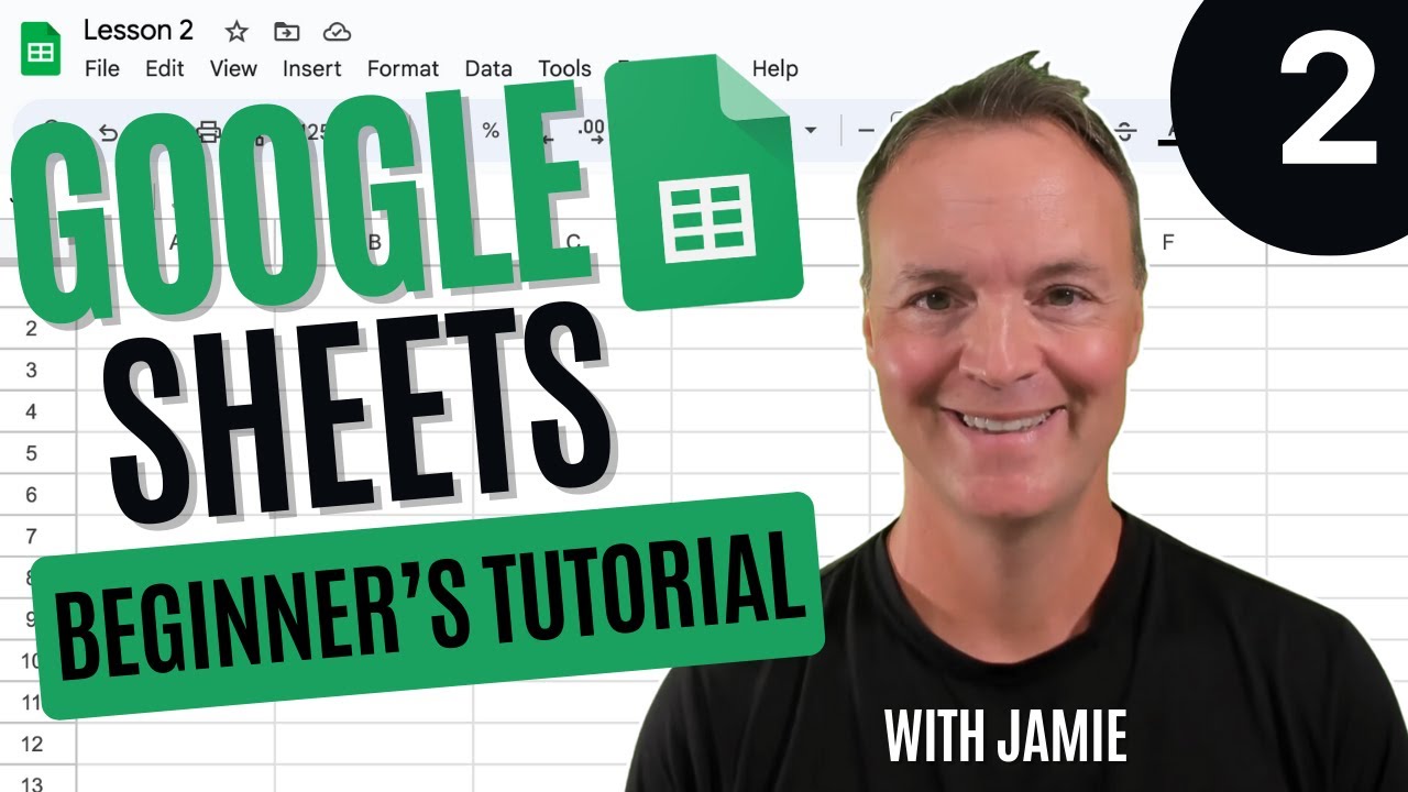
Beginners Google Sheets Tutorial - Lesson 2
Machine-readable: Markdown · JSON API · Site index
Описание видео
Welcome to Lesson 2 of our 'Google Sheets for Beginners' series! This comprehensive tutorial is designed to elevate your skills in managing and manipulating data in Google Sheets. Whether you're new to Google Sheets or looking to enhance your knowledge, this video covers essential techniques and tips to make you more efficient.
Practice Sheet: https://go.teachers.tech/GoogleSheetsLesson2
🕒 Timestamps:
0:00 - Introduction to Google Sheets for Beginners: Kickstart your journey into the world of Google Sheets.
0:43 - Autocomplete Data Techniques: Learn about the Fill handle and Smart Fill options for faster data entry.
6:11 - Upcoming Enhanced Smart Fill: A sneak peek into the advanced features coming to Google Sheets.
6:46 - Combining Cells - 4 Methods: Discover multiple ways to merge data in cells for better organization.
14:03 - Quick Text Splitting: Simplify the way you divide text across cells.
14:52 - Data Cleanup: Efficiently delete duplicate rows to maintain clean sheets.
15:59 - Cell Referencing Explained: Understand the difference between Absolute and Relative referencing.
20:15 - Transposing Data: Easily shift data layout for better analysis.
24:22 - Importing Web Data: Step-by-step guide to bring external data into your spreadsheet.
26:23 - Sorting Data Effectively: Organize your data for clarity and better insights.
28:26 - Sort a Range: Focus on sorting specific sections of your data.
29:46 - Creating Filters to Sort Data: Learn to filter and sort your data seamlessly.
31:51 - Creating a Filter View: Advanced filtering for collaborative work.
33:36 - Using the IF Function: Master one of the most powerful functions in Google Sheets.
Link to Movies: https://www.the-numbers.com/market/2023/top-grossing-movies
Links to Google: https://workspaceupdates.googleblog.com/2023/11/the-next-evolution-of-automated-data-in-google-sheets.html
🌟 Key Highlights:
Enhance your data entry with Smart Fill and Fill Handle.
Discover new ways to combine and split text for efficient data management.
Learn to clean up your sheets by deleting duplicate rows.
Gain insights into absolute vs. relative cell referencing for precise calculations.
Transform the layout of your data with the transpose function.
Explore how to import data directly from the web into your spreadsheets.
Become adept at sorting and filtering data to uncover valuable insights.
Understand how to use the IF function to make dynamic sheets.
✅ What You'll Learn:
Efficient data entry techniques.
Advanced data organization and cleanup methods.
The fundamentals of cell referencing.
Techniques for importing and managing web data.
Sorting and filtering strategies for data analysis.
Practical use of the IF function for decision-making in your sheets.
🔗 Related Videos:
Google Sheets for Beginners - Lesson 1: https://youtu.be/G93P4DxryVE