Welcome to our Intermediate Excel Mastery Series! In this comprehensive tutorial, we delve deep into pivotal Excel features and share insider tips to revolutionize your spreadsheet capabilities.
🚀 What's Inside:
✅ Master Pivot Tables & Pivot Charts: From basic setup to advanced layouts, learn everything you need to create dynamic reports.
✅ Uncover secrets of VLOOKUP: Step beyond basics with advanced applications and hidden tricks.
✅ Create Multiple Dependent Drop-Down Lists: A game-changer for data organization.
✅ Discover the power of UNIQUE Function: Effortlessly extract unique values from datasets.
✅ Implement Data Validation: Control user input with precision.
✅ Master a Nested FILTER Function: Combine with UNIQUE for ultra-precise data filtering.
🌟Perfect for All Levels: Whether you're a student, professional, or a passionate Excel enthusiast, this video series caters to all. Follow our step-by-step approach and apply these techniques to elevate your data analysis and presentation skills.
🔍 Detailed Timestamps for Easy Navigation:
0:00 Introduction to Advanced Excel
1:12 PivotTable Creation from Range/Table
2:16 Crafting Recommended PivotTables
3:01 Detailed PivotTable from Range/Table
3:55 PivotTable Fields: Adding & Reporting
4:50 Customizing PivotTable Field Layouts
7:20 Sorting PivotTable Columns/Rows
8:58 Integrating Filter Fields in PivotTables
9:59 Employee-Specific Report Generation
11:51 PivotTable Advanced Tips & Tricks
15:43 Integrating a PivotChart
19:02 VLOOKUP Function: Advanced Uses
27:42 Crafting Multiple Dependent Drop-Down Lists
29:42 UNIQUE Function: Data Extraction Simplified
30:40 Excel Data Validation: Techniques and Tips
32:03 Nested FILTER & UNIQUE Functions: Advanced Data Manipulation
35:58 VLOOKUP: Final Result Optimization
📈 Take Your Excel Skills to New Heights: Watch, learn, and transform the way you handle data in Excel. Don't forget to like, share, and subscribe for more expert Excel tutorials!
Practice Sheet PivotTables: https://bit.ly/PivotTable_data
Practice Sheet VLOOKUP: https://bit.ly/VLOOOKUP_data
Practice Sheet Multiple Dependant Drop-downs: https://bit.ly/Drop-Down_list
Check out this Intermediate Excel class: https://youtu.be/Ir22TLCjdto
Keep learning with these Excel classes:
How to use Power Query: https://youtu.be/MHIV0bYryiw
How to use Power Pivot: https://youtu.be/kyGhgreDNUQ
How to use the XLOOKUP Function: https://youtu.be/tPaXEZRh9_k
Drop-down lists with XLOOKUP: https://youtu.be/fjn4vlWwpCo
Drop-down with the INDIRECT function: https://youtu.be/oYF162_Cmwc
Excel beginners video tutorials: https://youtube.com/playlist?list=PLmkaw6oRnRv8lAKbKbflJRqS-9wuYNWUw
Function Lessons in Excel: https://youtube.com/playlist?list=PLmkaw6oRnRv_GeQNcc_hHtnxbRC7gDLST
- Hi there. Welcome to Teacher's Tech. My name is Jamie, and it's great to have you here. In today's video tutorial, we're gonna be taking a look at Intermediate Microsoft Excel. So, this is Lesson 1 in my Intermediate Microsoft Excel series, and we're gonna be covering three different topics today. We're gonna be looking at how to create a PivotTable with graphing, we're gonna be looking at the VLOOKUP function, how to be using it, and we're also gonna be looking at how to create a multiple dependent dropdown in Microsoft Excel. So, all these are gonna be timestamped down below so you can jump to different parts of this lesson. So, let's get started with the first one with pivot tables in Microsoft Excel. If you would like to follow along with today's tutorial, I'll put the links to the worksheets that I'm using down below in the description. Then you can click on the link, download, open them up, and follow along as I'm showing you in today's tutorial. Also, it would help me out a lot to know if these tutorials are helping you by hitting that like button or maybe even leaving a comment down below what you're looking for in future intermediate lessons too. So, make sure you do hit that subscribe button and that notification, then you get notified when my next tutorials do come out.
PivotTable Creation from Range/Table
So, we're starting with how to create a pivot table, and this is the data that we're using here. If you haven't downloaded this yet, just hit pause on the video, go to that link I mentioned before and download it and open it up. Now, to do an insert, it's very simple, you just go up to the menu and hit Insert. And below in the ribbon, you're gonna see pivot tables right away. As I go through these pivot tables, I'm gonna give you some tips and tricks also. And I'm gonna start with the tip right away. And the first tip is to select inside anywhere in the range or the table if you're using a table before you go and click on PivotTable because what it does, it automatically finds the range for you. So, here's an example. If I go up to PivotTables, notice that they have some recommended pivot tables here. I'm gonna cancel and click out and I click on recommend it again and it doesn't know. Now, I could still select my table or range from here and it'll be fine. But just as a quick tip, if you select inside of it
Crafting Recommended PivotTables
and pick PivotTable or Recommended PivotTables, it's gonna know where the data is coming from. Now, I just wanna mention a little bit about the Recommended PivotTables. This is a quick way to create them. Usually, they're pretty accurate with probably the main ones that you would want, but you can see where it goes sum of unit costs by regions, item. It does some recommendations based on the data and the titles that they think that you would want. So, you can always start with Recommended PivotTables and choose one of them, but we're gonna be going from PivotTable on it. So, and after we go through PivotTable, you'll understand after you insert the Recommended PivotTables, you can still make the same changes.
Detailed PivotTable from Range/Table
So, I'm just gonna go ahead, click PivotTable, and you can see that right away since I'm clicked inside of the range here that it has the sheet and the range from A1 to G44 here. Now, where do you want this pivot table to go? So, this is important, do you want a new worksheet or do you want it to be on the same worksheet? So, I'm gonna go New Worksheet and it's gonna open up another tab. You can choose what you wanna do on that or you can set a different location here. So, you can also choose whether you want to analyze multiple tables, and I'm not doing that in this case, but I'm gonna go ahead and hit OK and what you get if I look down at the tab at the bottom, you can see I have a new sheet right here and now they're asking me to start building my report by selecting my different fields to put onto it.
PivotTable Fields: Adding & Reporting
So, now we have to be selecting our pivot table fields, and you look over in the right and it can be done very quickly. So, if I go ahead and I'll just click on Sales Rep, and what you notice is it gets put into rows and now the names are gonna go down this column and then the data as I select it would be put into rows. You can quickly change this, so I could drag it into columns and now the names are gonna go across the top and we are gonna have our information below it in the columns. Now, we can quickly turn this off and on, the Sales Rep, so if I click off of it, it goes away. We can drag these down too. So, if I drag this into a spot, I could drag it around into columns, you can see how easy it is to manipulate. So, I have another tip here that I want to give you. So, this is kind of the default setup here with the fields down below where you drag into.
Customizing PivotTable Field Layouts
If you go up to the gear here and Tools and dropdown, you can pick a different way to view it. So, I prefer this one right here, I'm just gonna select it, and we get these on the side here with our different fields that we can just drag across. Now, that's up to you what you prefer. And the other thing I want to point out with if we go back to it, you can sort your fields A to Z. So, if you go ahead and select it, you can see how it changes it. Now, this if you had a lot of different fields, this would just make it easier to find them. So, just remember those couple tips right there. Okay, let's add some more things to this now. So, we're gonna have our Sales Rep here, and I want this in columns, and I'm gonna place it here so you can see some of the ones are hiding right now. And the other thing I want to add, so let's go ahead and add our totals. And you can see as I click on different ones how quickly it starts to change. So, I can click on and off. I'm gonna go ahead and click on Units. It shows all my sums of units here, but what I want is to have items. So, when I click my Items, now I do want this in rows, it places them down here. So, now if I pick my Units, it fills in so I can see each person. So, if I look at Dwight's, I can look at per binder, per desk, and all the different items, and it gives me the grand total there. So, these are just some different ways you can get some quick, your report being built by selecting the fields. So, did you notice if you click out of the data that the pivot table fields go away? So, click back in and they reopened here. Now, I wanna point out just if you're adding more fields, let's try, I'm gonna add a region here. So, if I click on Region, you can see it added to the rows at first and then it's gonna be breaking down this way, it breaks down the binder, and based on the central, north, and south where it was selling and being sold in different places. Now, if I bring this over to columns, you can see now that it's gonna go across the top. It's kind of breaking it between the different sales people. So, in the case of someone like Erin, you can see that she sold in the central and north while Dwight only here. So, go ahead, try different things, try adding by selecting different ones, selecting, seeing how it works to get the different reports on it and then moving from rows to column to see the ways you can adjust it.
Sorting PivotTable Columns/Rows
Now, another way you can adjust it is to sort, and if I look over here you can see that we have a dropdown, and this is gonna help me sort. So, in this case, this is gonna sort my column labels, which are the sales reps here, and if I drop down I can go ahead and select individual ones. So, if I said okay, let's deselect and I'm gonna go and let's compare Dwight, and I'm gonna compare Jim and hit OK. And you can see that we have the two right here and I can look side by side to see their totals of their items being sold. If I wanted to see total of amounts in different ones, I could pick a different thing to add from over here to add it. And you can see how quickly it can adjust. So, if you drop down again, I could select everything, hit OK, and everything goes back on. I can select this way too. So, if I wanted to sort a little bit more, if I didn't wanna see all the different items, maybe I just wanted to see paper, I could hit OK, and now I'm just seeing paper, and I see the salesperson so it makes it easy to look at that way. So, go and try a few different ways to sort. Now, I wanna show you how you can actually build an individual report and it will create a new tab down below for each sales rep, or depending on what you're creating, and it's done only with only few clicks. So, before I show you how to create a tab for each salesperson, I wanted to point out the use of filters. So, let's say in this data with the units, I just want to see by region also, and I like to filter through there.
Integrating Filter Fields in PivotTables
So, if I go and take Region and put it in Filters, you can see up top, I can simply now dropdown and I could be looking for a certain region or zone. So, if I wanted to see in central, I hit OK, and I just get those results back. You can also see that you can select multiple, so if you wanted more than one or switch it back. It's easy to add more than one filter, so or even move from different ones, I could take this sales rep here and move it up, and now I can sort by region and sales rep. So, if I was looking for, let's say, in the north, and I'm gonna also choose a sales rep, I'll choose Pam, hit OK, I can see in the north she sold this many. If I was gonna go back and check out a different region, at this point you can see now she hasn't had got anything in the south, so I just wanted to point out the use of filters. But now I wanna show you how you can use the filters to create a tab for each sales and person in this example.
Employee-Specific Report Generation
So, I'm gonna go ahead and deselect the items that I have here and I'm gonna build another report. And remember, I want a new tab for each one, for each salesperson. So, I do need a total, and this is gonna go into the values here. I do want the item there so I can see the item beside the total here. And we're gonna need the sales rep. And I'm gonna actually add this to the filter, so I'm just gonna drag it into the filter like this. Now, something else I wanna point out is to format your numbers here. So, if I go and just select in here, I can right-click and number format. So, maybe you wanted in accounting or currency, you can see the different examples that goes through. So, if I want two decimal places and to look like this, I'm gonna go ahead and hit OK, and you can see how it formats it. You can choose the format that you would like. The other thing I wanna show you is if I right-click on this, you can sort this. So, maybe I wanted from smallest to largest or smallest or smaller, I'll just go largest to smallest, just like this. So, some things that you can do to it. Now, what I want to do is generate the individual reports on each tab. If I go ahead and dropdown and go to Options right here, and you can see Show Report Filter Pages. So, when I select this, we're gonna get Show Report Filter Pages. If I go ahead and hit OK now, it's gonna go ahead and if I look at the bottom, so if I look, there's Andy's, there's Dwight's, there's Erin, I'm gonna get an individual report for each salesperson. And you could adjust it depending on what you want. So, I wanted to make sure you understood how you could do that very simply inside the pivot table fields.
PivotTable Advanced Tips & Tricks
So, I'm just gonna go back, you can see as I go through these different ones, I'm just gonna go back to the original pivot table that I was working on here and I just wanna show you a couple other things and some more tips. Now, let's say I was curious where this 2,135. 14 number came from. If you double-click on a number, so I'm just gonna double-click on this number, it opens this up and shows how that number was created by all of this information. So, that was by a double-click, it opened up a new sheet when I did it, you can see there's a Sheet16 beside it now. So, just try double-clicking on a number and it's gonna show you how it's even broken down more. Now, some other things I wanna show you with formatting, and usually things can be done in a few different ways. I'm gonna just show you if I go down to value here, right here, and just drop down, you can see that there's Value Field Settings. You can also get to Value Field Settings if you right-click on them too. You can see Value Field Settings right here. So, if I go ahead and choose value, this settings here, Value Field Settings. Let's say I could say an average account if I was doing a Count, hit OK. Well, the dollars don't make any sense anymore, but it's just counting up, here it would be 15 rather than $15. So, depending on what you were trying to show in your pivot tables, remember that we have value settings and you can change what you want right through here. So, I'm gonna leave this as Sum. Now, another thing I wanna show you when you're right-clicking is if you right-click, you can Show Values As. So, I find this is a cool way to show percentage. So, do we want, you know, you try a few different ones. So, if I say % of Row Total, Column Total, it'll say Column Total, I can see that the binders make up 48%, the pens will make up 21%, and it just shows you in a different way. So, all these different reports can be generated and remember, you're right-clicking to get to more of these here. So, I just go back to no calculation and it's gone. So, now I wanna show you how you can apply some conditional formatting to your pivot table numbers here before we get into the graphing and charting. So, let's say if we wanted this to be like a data bar through here. So, what I need to do is go back up to the Home tab up top here and look under Conditional Formatting. If I dropdown, you can see we can apply all these different things, but we're looking at the data bars, data bars and if I hover over, notice it's just doing the cell that I'm selected in and I wanted to be applying to all of them. In this case, just go to More Rules right here and you can see apply rule to only that cell. No, we want it to apply to that cell showing the Sum of Total Values here. So, if I select this one here, that will do the trick. Now, the other thing, do you want the numbers to be shown? So, right now we show both or do you want to be just the bar only? So, I can go and pick a color now and it will preview down below, so maybe I pick an orange just like that and I'm gonna go ahead and hit OK, and now I have a data bar applying to these different ones. So, just different way to show your reports that you can add conditional formatting to them. Okay, let's move over to graphing or charting our pivot tables now. So, let's say you wanna chart your pivot table report just to make it look a little bit better, a little bit easier for people to just take that quick glance and know what's happening. So, I'm just gonna select inside of this here and I'm gonna go up to Insert.
Integrating a PivotChart
And take a look, we have PivotChart right here. We do have the dropdown, I'm just clicking on it here. And right away, so it defaulted to the column. I can pick, I just got an idea maybe of different ones how it looks here just by going through. I'm gonna keep this simple, I'm going to create a pie chart here. You can see up top, if I wanted to see a different view, I can hover over to get the view to try any of these different ones. I'm gonna just keep it to the pie right now. Okay, so now just hit OK on it. And I have this in here, I can move it around, I can size it if I wanted to differently if you wanted it larger here. Now, I wanna point out this is dynamic so I can take a look at different things. So, if I wanted to take a look at the sales rep here, maybe I wanted to compare different ones, I could select multiple, maybe I just wanted to pick one. So, if I pick Michael Scott, I can see just the one person's here. So, it's going through, finding the information, and breaking it down for me. You can see the items or over here. So, if I go back I can go and select all and it puts it back again. So, you can sort using the chart to give those quick looks. I can dropdown here also, and if I wanted to maybe deselect if I just wanted two things here. So, if I had paper and desk, hit OK, and it just compares the two different ones. So, you can do all these different things within the chart still just like we were doing just with the data before, so but you can apply this to the chart. So, now what I wanted to show you too, you can make this, customize this look, if you just double-click in it. If this wasn't open, this Format Chart Area, just double-click on it and it will open it up. You can see I can quickly start to change things whether I want it to be maybe a gradient fill, you can see how the background changes. I can adjust my colors down here if I wanted to add different ones, if I wanted a pattern, pattern fill, you can play with all these different options. We have our text options also here. So, if you wanted to change different fonts and colors, you can adjust all those things. So, if I go ahead and select, maybe I wanted this to be differently, I can even dropdown, so that's the Chart Title. Or if I wanted maybe the Legend here, you can see how it selects different things. So, I could go ahead, maybe I'll add, I can change the fonts like this. If I wanted the legend to be positioned differently, I can start to change things all around. So, all these different things that you can play with to get the chart looking how you want. You can move these inside too, so if I wanted to place these in different places, again you can size your chart differently to get it the way you want. So, I hope you like this, this intermediate pivot tables. I'm gonna do more about pivot tables in future lessons just because there's more that you can do with this. I thought this would be a good start for you if you kind of just maybe touched the surface to them before or maybe haven't used them at all either. So, now we're ready to move on to our next section.
VLOOKUP Function: Advanced Uses
So, now I wanna show you how to use VLOOKUP in Microsoft Excel. VLOOKUP is a very powerful function that you can use to look up something in a column vertically, that's where the V is gonna come from. So, it looks down a column that you set 'cause it's gonna be the furthest left and then it returns some item in a that corresponding row. So, in this case here I already have VLOOKUP in this cell already created and I'll create a new one here. If I just go ahead and select this cell, you can see in the formula bar, it's already there, but what it's gonna go through, so it looks at GOTC right here and it finds it, I told it to go down the furthest left of the selection and this is this vertical column here. It finds GOTC, then I told it to look up in that row, this salary here. So, it gave me back 68,000. So, let me just change it, so instead of C, I'm just gonna go put I here, and it returned 58,000. So, it went over to the furthest left here, found the range that I selected and it went down and it found GOTI right here and it went across and found $58,000. So, this is a small data set here, and if this was a large one, you would probably see how much more powerful this is. But if you had thousands of employees and you're looking up something like this, with this formula you can simply just do those searches really, really quickly. Now, something I just wanted to point out here with VLOOKUP, I was just taking a look at the XLOOKUP function because XLOOKUP has a few more capabilities to it. With VLOOKUP you can only look to the right, but XLOOKUP you can actually look left or right. And with XLOOKUP you can kind of do the HLOOKUP or VLOOKUP together. So, it's something I would recommend if you have a newer version of Microsoft Excel, I do have a video tutorial on that, and I'll put a link in the description now below it and up and above in the card. So, let's go ahead and start our VLOOKUP and build it for this sheet. And if you haven't got this sheet open, hit pause, download it and follow along. So, we're gonna go through the VLOOKUP function a couple times, couple different examples in two different cells. The first place we're gonna put the VLOOKUP function is right in this cell. So, what I want to have happen is it's gonna look up an employee name and bring me back an employee designation. So, it needs to go over to this column here and then look down this column here to find that the designation in the same row that it found the employee name. So, we're gonna start in this one first time we're gonna go and just go Insert Function up here. So, open up that one, Insert Function. If you don't see VLOOKUP, just do a quick search. You don't need to type the whole thing here. I'm just gonna hit Go and then double-click on it. So, we get our four different arguments here. So, the first argument's gonna be the Lookup Value. Well, the Lookup Value is what the name is that I type into this cell. So, this is gonna be the look up cell or look up value in this cell right here. So, I'm gonna click in I6, and you can see it put I6 into there. The next is the table array. So, I'm gonna click in this spot and the table array is gonna be this selection. And remember, it's gonna be the furthest left column of that array that it's gonna search down. So, it's gonna look for a name here. And so, I need to make sure this is the furthest left column, and it is, so I'm gonna select here. And I need it to go to at least go to employee designation. It could go all the way to salary if I wanted, but it doesn't need to, but I'm gonna leave it right there for this one. Now, the next one is the column index, and this is how it works. So, in B, this is the first part of the table or range here. So, this is column one, even though I have A here, there's nothing in it, this doesn't count, so B is number one, C is number two, D is number three, E is number four, and F is number five. So, we told it to, it's gonna look down the furthest left of my array, that is this one, and I need it to look down what's the column I need it to search through? Well, it's gonna be D right here, and that's three because it's one, two, three, so I need to put three in here just like that. So, the next thing what I wanna do is type in a true or false or I could leave it blank too, but in this case I'm gonna type false and that means an exact match. If I put true, it's an approximate match, but I wanted to find an exact match in this case, so I'm gonna type in false like so, and I'm gonna hit OK. And it came back, notice it came back with N/A here, that's because I don't have anything typed in. So, let's just type in John here and we'll type John and it returns software engineer. So, went to the furthest left of the array that I showed that I selected and then it went to column three and found what was in there, so that's software engineer. So, if I go ahead and type Bran here, it went down this column, the furthest left, and then it searched column three and brought back analyst. So, this is working quite well. You can see it doesn't take a lot to create the VLOOKUP function. One problem is if you're using false, I'll show you the problem if we go to Bran here, and I'm gonna just click in here and let's say there's some spaces just like that. Notice it went to N/A? It's because we are looking for an exact match, and you gotta be careful not if you're using the exact match not to have spaces. So, as soon as I get back, I delete that again and hit Enter, you notice it works again. So, I just wanted to point this out. Okay, let's run through VLOOKUP one more time. So, I'm gonna go ahead and recreate the top one from up here for VLOOKUP. Now, the reason I'm gonna do this because it's a little different on how to count the column. So, I'm gonna go, what do I want to have happen? Well, the VLOOKUP is gonna go into this cell, so it's I10, and I'm gonna start my function this way this time just by putting the equal sign then VLOOKUP, and I'm gonna choose it right through here. So, what is my lookup value gonna be? Well, the lookup value is gonna be whatever I put into this, so this is gonna be the code, and I'm just gonna go ahead, click on that cell, I9, and comma. What's gonna be my table array on this one? Well, one is gonna go from the code up here to the salary one here, so there's gonna be four different columns in there. And then at the next point I'm gonna put my comma, what's my column index? And now, this is where things have changed. So, remember last time I said B was one? Now, that the array is starting here, this is gonna be one, so C is one, D is two, E is three, F is four. So, it's wherever the array is gonna be starting on it, so I just wanted to point that out. So, what do I need? This is gonna be one, two, three, four, so I have to put four for my number on it because this is not selected in it. So, I'm gonna go ahead, put my comma and then put my exact match again. And that should be all I need, I'm just gonna finish off with a bracket, and let's try this out. So, if I just put in GOTI, GOTI like so, and you can see that GOTI here was $58,000 here. So, I just wanted to point out when I was doing the VLOOKUP function this way is making sure that you understood when you count your columns, it's wherever the array starts, that's gonna be number one and then you move over from there. And then, if you have to go back and correct anything, you can just go back, you can either correct it up top here or double-click into this cell and it will open up. So, if you wanted to change this to true or false, so you can move those back and forth or change a different range too. All right, let's get ready to move on to the next section, and that's gonna be creating the multiple dependent dropdown list in Microsoft Excel. And I'm actually going to use a VLOOKUP function in that one too, I'll add that at the end. All right, let's go to the next one.
Crafting Multiple Dependent Drop-Down Lists
So, in this section I wanna show you how to create a multiple dependent dropdown list in Microsoft Excel. Now, there's different ways that you can do this, I actually have different videos showing different functions and formulas to create this. I'll put a list of those down below and you can check those out to see if those work better for you. In this one here today that you'll be working through, we're gonna be using the unique function and the filter function. So, what we're gonna do, I'm just gonna give you a little demo here to start with. And what it means is when we have a dependent dropdown list, what I choose in here will influence what I get over here. So, if I dropdown here, it shows the different departments. These different departments are being pulled from this column over here. So, if I pick finance here, then my list will change here, so it will change on what I can pick. So, there's only accountant in here, so I'll show you if I picked a different one. If I went to security and then dropdown, you'll see that I get head of security or the guard. So, if I was picking guard and then dropdown, I only have one person that's listed as a guard, but if I was going to go back and pick maybe let's say marketing, and then I was picking marketing assistant and then dropdown, notice that two people came up for marketing assistant, and then I could pick one of them and then their salary comes up based on what I picked. So, these were all dependent upon what I chose before, and that's what I wanna show you how to create today in Microsoft Excel. So, the first step here is to be able to pull out the individual market names here. You can see that there's two sales here, three sales, there's multiple marketing. I don't want it to be written each time, I just want sales to be once and finance to be once. So, I just want to be able to have all the different department names. So, what I'm gonna do is use the unique formula to begin with, and I'm not gonna put it
UNIQUE Function: Data Extraction Simplified
in this spot right here, I'm actually gonna just put it to the side here and I'm gonna start my formula here. I'm gonna be putting all my unique and filters down in this row, and then I'm gonna hide it after so you can't see it. So, I'm gonna go equals and then I can start typing unique. You can see as I start typing, it's closer and closer, here's unique, I'm gonna select it. All I need to do is select what I need to be searching, and it's gonna be this right here. So, I'm just using a range here. If you were using a table, you'd be able to select that column by the columns name too. But I'm just using a range, so I'm actually gonna just hit Enter, and I get my unique different department names. Now, this is what I'm gonna be putting in department over here, and this is where I need to use data validation. And where you find this is if you go up to the Data tab up top and then looking in the ribbon
Excel Data Validation: Techniques and Tips
find your Data Validation. So, I'm just gonna click on it and what we need to change it to is List, so Allow List just like this. And what is the list gonna be? So, I'm just gonna click on this, it's in this spot here, this is where the list is coming from, and I'm just gonna hit Enter. And I'm gonna show you something, I'm gonna make a change to this so it works better in a moment, I'm gonna hit OK. And watch this what happened, so I dropped down, notice it only says sales on this? What I could do, I could have selected everything so it would've shown everything. But what I like to do is, and I'm just gonna click on Data Validation again and open it back up. If you add a hashtag at the end, it will always adapt to how many spaces is in that list that it's pulling. So, if I hit okay now and go back, you can see that all of these from here are now in my dropdown list here, so this is the first step that we're gonna do. So, the next step that I want to have happen, I want to be able to once I choose sales, then I should be able to only look within the sales job titles that are there. So, it should look down this list and there are repeats of different ones, you can see there's sales assistant, and sales manager, so it should find two different things. So, I am gonna be using unique, but I also need to filter it
Nested FILTER & UNIQUE Functions: Advanced Data Manipulation
and I need to connect it to this H2 cell. So, let's go ahead and start our unique function formula over here. And to do this, I'm just gonna put equals and then start typing unique, and I can see it pop up, but right away I need to add the filter function. So, if I start typing filter and I need to add this, and what do I need to be looking at? The array, so I'm gonna be comparing this and I'm just gonna select the whole column here. And then I'm gonna put a comma, it's gonna be comparing to this one here. But when this one equals what? Well, this is where I need to put the equals sign in of the plus equals, this spot here. So, I was gonna look down C to see when this connects to here. And then that's the end, so that's one bracket, we have to add another bracket 'cause we have the two opening ones there too. So, I'm just gonna hit Enter, and you can see since I have sales now it brought back sales manager and a sales assistant. If I drop down and go to marketing, it brought back these two. Now, we're gonna do the same thing what we did before, we are gonna put the data validation, data validation up here. So, I go to this spot, I click on Data Validation, and what am I gonna use? Well, I'm gonna use a list again, and what's my source gonna be? So, I can click on this and I'm just gonna click in this cell here and I'm gonna add the hashtag right away, hit Enter and hit OK. So, now we should have this, marketing manager, marketing assistant, it's pulling from here. So, if I change this to finance and look what we have, there should only be accountant, and you can see it reflected over here. We'll make one more change to make sure it's working, security, and now we should have this dropdown between head of security and guard. Okay, let's move to our next spot. So, now we want the names to populate down here based on the guard. So, like if we have this selected, it should just choose the one guard that we have, the name list. So, how do we do this? Well, the names are all unique already, so we don't have to use the unique function in this one, we'll just use a filter and connect it back to the H2 spot or H3 cell that we already have. So, I'm gonna go back to my J column and I'm gonna put in equals and we'll use our filter here. And what is it that we're gonna be needing? Well, I'm gonna need this column right here. And what's gonna be the next one? It's gonna be the job title. So, it's when the job title is equal to what? Well, whatever's in this cell right here. So, now I can go ahead and just close that, and you can see there's the one name. So, let's see what happens up here as we choose if we choose marketing and we choose, let's say, marketing assistant, we should have two names right here. So, it's pulled the list though. Now, we have to use our data validation to put it back into the dropdown list here. So, I'm just gonna select this cell, make sure you're under Data, go to Data Validation, drop down, choose your list. Choose your source, it's just gonna be this spot here. I'm gonna add my hashtag, hit Enter and hit OK. So, now I should get those two here. So, we have one more step here that we want to add and we wanna be able to connect their salary here. And we're gonna do this actually with VLLOOKUP, sort of similar to what we did in our last lesson. Now, let's use our VLOOKUP function to finish this off by getting the salary connected to the name. So, our function's gonna go in this cell right here in H7
VLOOKUP: Final Result Optimization
and we're gonna start this with our equal and we're gonna look up for VL. And there it is, I'm gonna select it. So, what are we looking up? Well, we're gonna look up what name is in this cell right here. So, I'm gonna select it, that's why I look up value, place my comma. What's my table array? Well, my table array is gonna be going from this part up here at the beginning of the names down to the end of the salary here. Now, our next point is our column index. Now, remember, since employee name is the first column, this is number one, so this is the first column in the array, this is one, two, three, four. So, we're gonna need to have the column index number B4, so I'm gonna put in number 4 like that, and I'll put another comma, and I want it to be false because I want the exact match. And I'll just end this and hit Enter, and let's try it out a few times. So, if we're dropping down here, and if I was looking in sales dropdown, maybe I wanna see sales manager and dropdown here and I can see Walter White gets $186,556. And the thing I'm gonna point out now, you can see all these things changing in the column J. You can hide this, so what you can do if you right-click at the top of the column here on J, we do have Hide here. So, it didn't delete it, it just hid it there, so now people won't see the information coming up there and then you have your multiple dependent dropdowns working right through here. And then you have the VLOOKUP function getting that salary from reading this last cell. So, like I said before, there's many different ways that you can create multiple dependent dropdowns in Microsoft Excel. I do have other ones, I like the XLOOKUP one too. You don't have anything to hide in cells, so take a look at that one and I have some other ones too. I'll put the links to those, as I mentioned, down below and in the cards. This brings us to the end of this Intermediate Microsoft Excel Tutorial. Make sure you keep posted for when I have the next ones coming out, and check all the links down below in the description to all those other tutorials that I talked about. Thanks for watching this time on Teacher's Tech. I'll see you next time with more tech tips and tutorials.