PyDMD: A Python Package for Dynamic Mode Decomposition (DMD)

Hi everyone. Uh so my name is Sarah Ichinaga. Um I'm from the University of Washington. Um and today I'm going to be talking with you all about the Python dynamic mode decomposition or PIDMD Python package. Um I come to you all as one of the many contributors and also current uh maintainers and developers for the PIDMD package. And I'm really excited to be talking with you all today about basically what PIDMD can do, how you can get started with it, and how you can use PIDMD to start analyzing your own data sets. Uh so let's go ahead and get started. So before we dive in though, I just want to review sort of what this video is going to cover. Uh so first we're going to start with some introduction and motivation. basically answer the question of uh why do we uh build mathematical models in the first place and why would we want to use methods like the dynamic mode decomposition um then we're going to get into a little bit of mathematical background basically just review very briefly um the dynamic mode decomposition or DMD algorithm basically talk about what does the algorithm do um and what kind of information does it provide us with um and then after that we're going to jump straight into the code uh we're going to basically talk about how you can use PIDMD to apply by DMD in practice. Um, and this portion of the video will uh include a coding demonstration. This uh this material will take up the majority of the video. Um, but yeah, so that's about everything and I guess the before we kind of get into specifics, I just want to point out that this tutorial um along with many other tutorials will be available online at the PIDMD GitHub repository found at this link. So if you are interested in reviewing the materials later or learning more about PIDMD, I highly recommend you go here and check it out. Uh so yeah. Okay. So some motivation starting with motivation. Okay. So on the screen here I have a few examples of some real world time varying snapshot data. You know these are just a few examples. You can imagine that there are many other systems that I could have put here instead. But the main thing that I want to illustrate with these is this idea that for many many scientific and engineering disciplines time varying snapshot data is abundant and readily available a lot of the time. Basically the act of collecting this for many disciplines is actually the pretty doable part. Like for example if I'm studying a an evolving fluid or if I'm studying some kind of mechanical moving system there's a good chance I can maybe take a video of it for example. Um, if I'm studying, for example, the temperature of the ocean and I want to understand how that evolves in space and time, I can collect that data. I can collect the temperature of the ocean at various points in space and time and then I can get data sets kind of like this one right here. Um, however, although we have access to a lot of data sets like this for many fields, the problem is for many of these systems, we don't actually know the precise set of governing equations that describe these systems, right? Like for example, we don't actually know for example how the time derivatives of the temperature of the ocean will change precisely as time goes on, right? We don't actually have precise equations usually. Um but we would like to have precise equations a lot of the time because if we had access to governing equations, we could say basically a ton about our system. We can make future state predictions. We can understand how external forcing or inputs might affect a system. you know there's a lot we can say and we would like to know these equations but and so basically this um motivates the question of given access to time varying snapshot data can I somehow leverage that data and use it to craft mathematical models that can allow me to do a variety of useful tasks and help me better understands understand the systems that I'm observing right so this is the goal of what we're trying to do um and so what do I mean when I say build a mathematical model so let's take this fluid flow past a cylinder data set as our main example for now. Um, and let's say that this is the system I'm observing. I've taken I've gotten snapshot data of it. Here's my video. This is my data set. Okay. Um, and so really for basically all video data, you can really just think of this as um a collection of snapshots um right or a collection of frames, right? And I can think of every frame of this video as an observation of some state variable. I'll call it X. And a video is just an observation of X at time one, time two, time three and so on. And essentially this is what I have access to this data here. Um and what I would like to do or the goal when we say find a mathematical model is this idea of I want to find sort of a function f such that when f acts upon my state given by x, I want this to sort of give me a really good approximation of the time derivatives of the state. If I have access to f, I have my governing equations. I can make predictions. I can do all the things that I want to do. So this is the goal finding f. So how do we go how do we actually go about doing that? Um so that leads us to talking about the dynamic

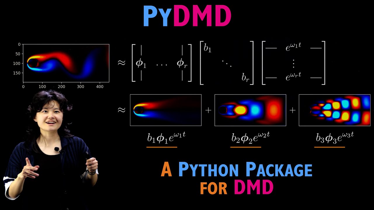
mode decomposition or dmd algorithm. So dmd is just one of many ways that you can go after the function f. It's certainly not the only way. Um, but for reasons that we'll get to later, um, DMD is actually DMD actually provides us with like one of the simplest sort of mathematical models or functions f that we can possibly get. Um, and so it's sort of one of those things where if DMD works for your data, it's kind of like why not use it? It's super informative and it's super simple in terms of the model that is. Um, so but before we sort of address why that is, let's go ahead and talk about the algorithm itself. Um, so DMD uh starts with you building a data matrix X. Okay, where the columns of this data matrix X contain your snapshots of the state. Okay, and so if we're still going off of that sort of fluid flow pasta cylinder data set, you can imagine that every column of this data matrix is going to be a frame of that video um every snapshot uh from that um video, but basically flattened into a vector so that these snapshots can fit within the columns of this two-dimensional data matrix X. Okay. Um once we uh make our data matrix X in general DMD seeks to find a decomposition of X with the following form. There's three major components to this decomposition. I'll kind of talk about them one by one first. So the first part of this decomposition is um this sort of spatial mode matrix um fi and we call it that because the columns of fi actually turn out to contain what we call the spatial modes or the dominant sort of spatial sort of features of the data set. Okay, the next one that I want to draw your attention to is this uh time dynamics matrix t uh parameterized by omega. And you sort of look at this matrix defined on the over on the far side over here. Essentially, every row of this matrix is a time series defined as an exponential raised to some corresponding frequency. As we go across the columns, time increases from time t1, t2 all the way up to our final time um time point. Um and each row is parameterized by their own sort of um omega value. Um and so depending on what omega is, these time series can oscillate. They can exponentially grow. They can decay totally depending on what omega is. And when we perform DMD, we're trying to figure out what omega should be. Okay. Um and then the final component is this amplitude uh matrix or these amplitude values I should say uh B1, B2 all the way through BR. And these are going to tell us sort of the prominence of the spatio temporal features given by DMD. Okay. And so, you know, I'm sitting here and I'm saying spatial temporal modes and like a lot. And so, you know, but what even what does that even mean? So, let's kind of talk a little bit more about that just gain intuition here. So, suppose I have my fluid flow pasta cylinder data set. Okay. And I perform DMD on it and I get this decomposition right here. Um, so this uh decomposition, this is exactly like what we had on the previous uh slide just for reference. But really um one way that you can think of it is you can alternatively express this decomposition as the summation that I have written over here um and if you sort of look closely at it um essentially this summation it's a summation of r um it's a sum of r sort of pieces and the i sort of term in the summation has its own um spatial mode vector fi ii. it's being um and here we're applying essentially an outer product of fi with the exponential time dynamics defined by the i frequency value omega i and then all of this outer product is then scaled by the amplitude b and so essentially this is why we say spatial temporal modes every term in the sum is some outer product of a spatial mode spatial of the spatial features uh with corresponding temporal sort of um activity ity. And so this is describing essentially the E kind of set of spatial features that have their own sort of time variations. And then B is sort of then telling you because B scales this whole thing. It's then telling you sort of how important is sort of this spatio temporal mode in reconstructing this data set. Okay, the bigger the B, you know, the more that this contributes to the sum. The smaller the B, the less. And so it kind of gives you also some sense of hierarchical sort of spati temporal mode importance. And so more concretely if we sort of take a look at these individual terms after applying DMD to this data set what we find is that these spatio temporal modes when visualized look like this. And again DMD is telling us that this data set can be decomposed into a sum of our spatio temporal components where we have this spatial temporal component added with this spatio temporal component etc etc. This is thus giving us some kind of intuition for what are the dominant sort of spatial features and how do they vary

in time and how do they what basic sort of make up this data set right here. Okay. So all right, awesome. The final thing I do want to say about DMD before we move on is this idea that when you perform sort of a de a decomposition like this, when you make the assumption that you can express your data like this, you are actually sort of inherently assuming that the dynamics of your system are linear. What I mean by that is we are assuming that the time derivatives of the state are given by a linear operator times the state. And when I say linear operator, I just mean a matrix. A is just a matrix. Um and essentially the easiest way that you can kind of see or like the most intuitive way you can see that is if you can write the igen decomposition of the matrix A as the following. Um we actually know the solution to the system of differential equations analytically. We know it to be given by this. And if you sort of like offline kind of take a look at this sort of expression as um compared to the DMD expression, you'll find that this is exactly the same as the representation given by DMD. So again on top of sort of like um in an intuitive sense DMD tells us about spatial temporal modes that uh make up the data set but also you are literally finding a linear operator a such that a times the state is approximating your time derivatives of the state. All right so that is DMD in theory. Uh but what about in practice? Okay. Um so when you're applying DMD to your own data sets um it's totally okay for you to implement DMD yourself. Uh but I would like to point out that within the PIDMD Python package um there's already um implementations for a huge variety of DMD variants um extensions and also optimized algorithms. And on top of that, PIDMD also has data prep-processors and plotting tools. And so really when you if you use PIDMD to apply DMD to your data sets, it really just boils down to the following process. really just uh define a module that implements uh the DMD variant that you are interested in applying. Um you can then wrap your model in a data prep-processor if you would like to use one. Um you can then fit your model to whatever snapshot data X that you have. Um and then you can call a plotting tool from the plotter library and you can use that to sort of visualize the results of whatever DMD um process that you did. Um and really it just that's the whole that's the whole thing. Um, I also want to point out that PIDMD is constantly evolving because of work uh done by researchers in the field and so and we actually recently revamped the PIDMD package to contain new modules, new extensions, new algorithms and also some more tutorials. And if you're interested in sort of taking a look at sort of the recent work that we've done to revamp the PIDMD package, I highly recommend you read our recent journal of machine learning research paper um given down here. Uh but yeah anyway so given that let's go ahead and sort of dive right into the coding demonstration. So in this coding demonstration, we're going to be taking a look at um a synthetic data set that consists of these two uh spatial temporal modes given at the top right here. Um and we're going to show that using DMD and specifically PIDMD, you can take noisy signals like this one down here, this red signal at the bottom corner. You can take that and you can use DMD to recover the fact that this data set is um it's comprised of these two um spatial temporal modes. So let's go ahead and take a look at that. So let's open up our code. Um, nice. Okay, so we got the code pulled up now. All right, awesome. Okay, so this is going to be this is the Jupyter notebook that goes along with this um coding demonstration or this tutorial um and we're going to walk through it. There's a lot of um again this is going to be available on the uh PIDMD GitHub um in case you want to look at it later. Um there's a lot of uh documentation kind of walking you through like this notebook in case you would like to go through it independently but we are going together. Okay. So um first things first when you are applying DMD or applying PI DMD I'm sorry. Um you first need to import PIDMD. Um so there's a lot of ways you can do this. Um there's basically uh we do Pippi releases every month actually. But because PIDMD is constantly um evolving and sort of getting updated because research moves very quickly, um I personally would recommend that if you are installing PIDMD, you do so from the source code on GitHub. Um there's many ways you can do this. Um one of the easiest ways is to simply pip install with the git extension. And that is actually precisely what this line of code is going to do. And so I'm going to just go ahead and start off by running this so that we can import uh all the new PIDMD code. We're gonna Oh, yeah. Okay. So, that's going to go ahead and run. I'll just wait for that for just a second. Um, but the first thing we're going to do, um, in this notebook is we're going to define our synthetic data set that we're going to be playing with.

Um, and so essentially, um, but before we actually define the math math, we need to start with Oh, wow. Look at that. Look at it go. We're going to start with some essential imports. Uh by importing um numpy uh for computations and we're going to be importing um mapplot liib for uh visualizing results and we're also going to be defining an error computation function so that we can sort of uh get a handle on exactly how well DMD is able to reconstruct our input data. Um so let's go ahead and run that. Awesome. So we've imported. All right. So specifically, so let's get into some specifics. So our data set is going to be given or the clean version of the data set is going to be given by this function f of x and t. x denotes space, t denotes time. Um and f is going to consist of sort of like the contributions from both an f1 component and an f_sub_2 component. f_sub_1 will be uh defined to have a spatial component defined by this hyperbolic seeant function here. And it will also have time dynamics given by this exponential raised to 2. 3 I. Um as time goes on. Um take note of the fact that this exponential is only raised to an imaginary component. So these time dynamics will be purely oscilly. There is no real component that E is being raised to. So there will be no exponential growth or decay. Uh just oscillations defined by this 2. 3. Okay, keep that in mind. It's going to be important as we move on. Similarly, f_sub_2 is defined to have its own sort of uh spatial sort of um sort of structure and its own sort of temporal oscilly dynamics, but this time but for this one it's given by 2. 8. Okay. Um there's a lot of stuff in writing but I will actually go through the stuff that's in writing. I will actually say it out loud as we go through the code together. Um let me see maybe what no that's not okay. Yeah, I think the code is Yeah, code's good enough. Big enough. I mean, all right, let's go ahead and go through this. So, basically f1, here we go. We have a function f1 defining um our f1 com our f1 sort of contribution given um a spatial and a temporal grid. Uh we do the same for our f_sub_2 function. Um and then here as we go down, this is where we are going to be defining our data. So first we're going to say okay let us use let's use 65 evenly spaced collocation points in space and let us also use 129 evenly spaced collocation points in time. Okay. Um we are specifically going to be recording our data along this spatial and temporal grid given by this chunk of code here. Specifically we're going to be looking at values of x going from -5 to 5 and we're going to get 65 of those grid points evenly spaced. And we are going to use a temporal grid going from zero all the way up to four times pi using again evenly spaced time points using a 129 collocation points along the grid. And there we go. We feed the spatial and temporal grid to our f1 and f2 functions so that we um so that we define the contributions of f_sub_1 and f_sub_2 and x1 and x2 uh respectively. And then x our clean data matrix is going to be given by uh the contributions of x1 and x2 combined. Okay, so that's our clean data. For a little bit of added realism, we're going to be adding uh actually a kind of significant amount of Gausian noise to this data. Just for the sake of demonstration, we're going to use a noise magnitude of 0. 2. And we're going to take that and multiply it by Gausian random noise of mean zero. We're also going to ensure that there's an imaginary and a real component of this noise because the data set itself has real and imaginary components to it. Um, and then we're going to take that noise, add it to our clean data, and that is what we're going to define as X noisy. Okay, X noisy is what we're going to be giving to our PIDMD model. All right, awesome. And then here we just have some code that's uh for printing out some uh some sort of array information. But let's actually just go ahead and run this and sort of take a look at what this is going to generate. And so down here we have uh information on our spatial and our temporal grid as you can see. uh but in addition we are defining specifically uh this sort of x and t sort of numpy arrays with certain shapes. T is holding on to the times at which we collect our snapshots. But the main one I want you all to sort of keep in mind is the shape of our data matrix x. Note that x noisy is also going to be the same shape. Uh but the thing that I want to highlight here is this idea that x has 65 rows and 129 columns. Recall from our discussion previously, this is because we have 129 sorts of snapshots of our system. And for every snapshot of our system, we have in our case, we have 65 entries, 65. Why? Because we have 65 collocation points in space. We have 65 essentially features or variables for

every snapshot that we have. Okay, so that's something to keep in mind. uh this is how X is going to be structured not just in our theoretical discussion but also as input for PIDMD models. All right. And so uh before we kind of get into uh applying PIDMD or DMD to this data set, we're going to u first visualize this data set along the spatial and temporal grid, let me go ahead and actually expand this so that we can see it a little bit better. Um yeah, so pretty much let me actually also scroll up just a bit. There we go. So, um, here we go. We have some plots of our data of F1, F_sub_2, our clean data set, which is F1 plus F2, and then our noisy data set over on the far side. And so, what I would like to point out is that this is a visualization of the whole shebang. This is all of our data across the entire spatial and temporal grid. This is giving us an overview of like what this data set looks like entirely. Um, along this axis here, we have our space, uh, our collocation points in space. Note that we're going from 5 to 5 as expected. And along this axis, we have the time axis. So we are going from time 0 all the way up to four * pi. And this is literally visualizing what f1 looks like across time and space. This is visualizing what f_sub_2 And so on and so on. This is what our data looks like on the grid. But it also is still a little bit it leaves a little bit to be desired. I would argue this doesn't really give us amazing intuition for what this system is actually doing. Uh which is why in the bottom cell right here I've provided some uh movie pi code to generate sort of uh video versions of this data set. I will not be running it because sometimes movie pi can be a little bit finicky at times. But I will be showing you all a video uh that I have generated previously for this data set. And let me just go ahead and Okay, I think yeah. So I'm going to zoom out for just a second. Some kind of formatting here happening does not like my shape sizes. Okay. Yeah. So if I go ahead and play this video which is the same data set that we had visualized before just in video form. Um this is exactly what our data sets look like. So along the horizontal axes now we have um space our spatial collocation points X and what we are literally seeing is f1 f_sub_2 our data and our noisy data but seeing how they vary as time sort of progresses like visually um let me just go ahead and play that one more time for you guys. Let's see I will stop talking for a moment just like let you all take in what is going on. Okay. Um and actually so and like the thing that I want to point out is this idea again I will continue to emphasize this idea of spatio temporal modes in the data. Essentially we can think of f1 as its sort of spatial signature is the sort of hump that kind of goes like that kind of exists in this area here and it sort of moves in and out at its own pace which we should note is precisely defined by that 2. 3i that we used to define this data set. Right for F2 it's a little bit different. Its spatial signature is a bit different. And it's got this little uh let me do Yeah, sort of double hump sort of spatial signature and it is kind of pulsing in and out at a actually different frequency that's defined by that 2. 8 I right and so you know these two sorts of features with their own spatial signatures and their own uh time signatures are being added together. we're polluting it with noise and we are basically saying can we use DMD can we use basically DMD to kind of reverse this process and figure out from noisy data that these are the two sorts of main components of this data set. Okay. And let me play that one more time. And you can kind of see like the noisy data set. It looks pretty confusing actually like but I will but I would like to emphasize that is what DMD spoiler I guess DMD will be able to do it but anyway let's go ahead and sort of show that in action. Um all right so let's go ahead. All right. So that is the data set that we're going to use. Now let's actually start um applying uh DMD with pi DMD. Okay, so this is all the math that we discussed uh previously. I'm not going to go over it again. This is just for uh reference for this notebook. But if we kind of scroll down, this is where we're going to start putting in sort of our PIDMD code. Um okay, so PIDMD is structured very modularly. So uh it's really similar to the way uh scikitlearn is sort of um sort of structured in the sense that you have objects or modules that implement uh methods. uh you initialize those you parameterize them and then you call a fit method and then once pass data through that fit method then there's attributes that will be available to your model so just for anybody who is uh

familiar with scikitlearn uh style sort of syntax or like um machine learning uh that's just something to keep in mind when using pymd it's a really similar situation um so that kind of leads us to and that leads us to talking about the first thing which is first we need to decide what DMD uh model we want to use or what method do we want to use. Um so uh there's a ton of variants out there. Uh the task of choosing a DMD variant can be quite daunting. Uh but in general um personally I highly recommend for just normal DMD applications uh that you opt for what is called the optimized DMD um algorithm or um another sort of related and slightly more sophisticated version of optimized DMD is BOP DMD which uh stands for the bagging optimized DMD algorithm. Um, it is a very noise robust optimized variant of the dynamic mode decomposition that is incredibly practical and is able to apply DMD on very uh noisy data sets. It is um it works even with unevenly spaced snapshots. That's not an issue here, but it's something to keep in mind. And so in general uh when applying just um more typical or just um sort of any DMD application in the real world it's the uh method I would recommend. And so if you want to apply bop DMD with PIDMD uh it kind of boils down to first uh importing the right module. So from PIDMD you want to import the module you want to use. So bop DMD is um as you might guess is implemented by the bop DMD module. Um then once then the next thing you need to do just like with scikitlearn type models uh you need to initialize your model and parameterize it. So again recall so our toy data set consists of two spatio temporal modes. Um and what we would like to do is kind of say well I want to apply DMD but also I want to take into account the fact that there are two uh sort of dominant spatial modes sort of in my data. Um let me just go ahead and move this over to the side here. Um okay and so uh we can kind of do that by sort of passing in some parameters to our bop DMD model. So, uh, what I'm going to do is I'm going to call my bop DMD pi DMD model. I'm going to call it just a lowercase DMD. I'm going to initialize a bop DMD model and then I'm going to parameterize it with SVD rank is equal to two. Now, what this is going to do is it's going to tell uh my bop DMD model, hey, I am anticipating two spatio temporal modes. Okay, that's how many I want you to learn as we go throughout computing uh DMD. Okay, so that's what that means. And then once we build our model then all that remains is to fit our model to some uh snapshot data. So specifically you need to invoke the fit method. Basically every pymd module uh implements its own fit method. Um and sort of goes about that differently depending on the variant. Uh so here we're going to call fit. Um this is going to perform the bagging optimized DMD routine. Um and then we need to give it our snapshot data. Specifically we are going to give it the noisy snapshot data that we have. And then also Bob DMD requires that we give uh we also provide uh the times [clears throat] at which we have collected our snapshots and that is stored within the time vector t that we defined. Okay, so I'm going to go ahead and run that. Um okay, and so it's going to give you a little warning. Um it's okay um to sort of disregard it for now. Sometimes uh the bop dmd uh implementation can be a bit picky about tolerances with its optimization and so it'll maybe throw this warning. But um sometimes and actually for a lot of cases um even if this warning goes up your fit is actually ends up it ends up being pretty all right. So I wouldn't really worry too much about this. Uh this is just kind of and this is kind of showing us okay so now we have a bop DMD model from pi DMD. So now what exactly are we working with now that we fit this model? Okay, so the first thing I want to point out is just and again just like really similar to scikitlearn models now that we've done fitting we have now have access to model attributes uh specifically if we recall with DMD we have those three attributes remember we have spatial modes uh frequencies that define the temporal um frequency and the time dynamics matrix and then we also have amplitudes B okay so let's kind of see how do we get all three of those components from a fitted PIDMD model so to get the frequency ies you just need to you can access all of that through the IG property. This is now going to contain something now that we've fitted our model. But if I run this uh you can see that what this is going to hold on to is basically a two element array uh that contains our igen values. We call this uh the property is called iigges because these are quite literally the igen values of the continuous time operator given by a which describes the uh the um derivatives of the state. Um but also these are also those omega parameters for our time dynamics matrix. Okay, those are those omega one and this is like an omega 1 and omega 2. Okay. Um and you know we

have two frequency values. I want to point that out. Why two? Well two because we asked DMD when we built our model, hey I want to build two spatio temporal modes. And so um as a result we're going to have two frequencies one for each spatio temporal mode. Okay. And let's kind of take a closer look at sort of like these elements here. So um if we kind of zoom in on the real components of these, we're going to see that these real components are very small. They're like something like something* 10 theus4. You know, they're very small. But if we take a look at those imaginary components, what do we see? We see one of them is 2. 79. So approximately 2. 8. And then the other one over here is uh 2. 29, which is approximately 2. 3. So does that seem a bit familiar? Um yeah. So you'll notice that when we apply DMD um to this data set, we are finding uh frequencies with very small real parts and with imaginary components that correspond directly with sort of those frequencies that we use to parameterize those exponential time dynamics for the true the underlying ground truth spatial temporal modes. Right? So if we kind of go all the way back up here, I'll kind of show the equation just one more time as a like just to refresh on this. This is precisely related to the fact that we defined f1 and f_sub_2 to be there are time dynamics to be parameterized by these um 2. 3 * i and 2. 8 x i sort of components. And so what we are finding when we apply DMD is we are literally um sort of discovering that from data alone, right? Um but this is the first component. Now let's move on to some more components. The next component that I want to look at once you fit a DMD model, you now also have access to uh a modes and a dynamics um attribute. And so what modes is modes is literally going to be that spatial mode matrix 5 that we were just talking about. Um and the dynamics attribute is going to be essentially that t omega matrix. It's that um matrix of exponential time dynamics parameterized by those IGEN values we were just looking at. And it's also going to be scaled appropriately by the amplitudes B. And so uh to get more intuition on this, let's go ahead and actually print this out. So let's or let's start by printing out the shapes, right? So like I'm going to say dmd. modes and then we're going to print just the shape. We're going to do the same thing with the dynamics. DMD. damics uh shape. Okay. And then let's go ahead and run that. All right. Cool. So these are the shapes of these two uh properties. Um and let's kind of take a look at this. So modes is going to or in our case modes is uh a matrix that contains 65 rows and two columns. Two columns because we have we asked for two spati temporal features and therefore or two spati temporal modes and therefore we have two sets of spatial modes that we care about. Um and then each of those modes has 65 features. uh 65 features because that is precisely how many spatial collocation points uh we are dealing with. Okay, so that's where the 652 comes from. And then for the dynamics shape, we have something that has two rows and 129 columns, 129 columns because that's how many snapshots we are that we have from our data. Um and so we have to account for the dynamics of all of those points in time for our snapshots. And then also there's two rows because we are accounting for the dynamics one set of dynamics for each uh spatial temporal mode. Okay. Um those are just the shapes but like uh you know given all of that context we can just go ahead and gain even more intuition by just plotting these out. So let's go ahead and do that. So um you can actually plot so since we know what our kind of collocation points in space are I can plot the columns of fi or the columns of the modes matrix against uh the spatial collocation points and so we're going to do exactly that. So dmdodes we're going to grab the first column plot its real component. So there we go. We're going to take the modes again uh grab the second um column this time and als and again plot its real component. These are going to plot literally we are literally taking the columns of phi and then plotting them out and seeing what they look like. Okay. And we're going to do a similar thing with the dynamics. Uh it's just that for the dynamics we want to plot it with respect to time. Okay, not space but time. And so then we're going to say, okay, give me the DMD dynamics. Okay, we're going to plot the first row and the real components of that first row. So like that first sort of exponential time trajectory, the time trajectory for that first spatial mode. And then we're going to do the same thing but for the second one. So D, oh D mix one, the second column, the second row, I'm sorry, and then the real component. And before I go ahead and run the cell

I also just want to point out exactly what else um is going on in this cell. So here um I'm going to be plotting in addition the sort of hyperbolic um trig functions that we use to define the spatial sort of um the spatial features for our underlying ground truth modes. So that's the first thing. Um and then I'm also going to uh be plotting some sinosoidal functions specifically cosine functions that are defined using that 2. 3 and 2. 8 sort of frequencies that we are using to define our exponential time dynamics for again for our ground truth dynamics. So we're just going to plot these. This is all going to appear on the bottom uh just for reference. But let's just go ahead and run this and see what it actually looks like. Okay. Nice. All right. There we go. Amazing. Okay. So what are we looking at? So let's break it down. So this first row is uh show sorry showing us basically the results from DMD. Again DMD is it only looks at the noisy data nothing else. It just sees that noisy data and uh the time points and then it extracts this information. Down here are sort of those spatial signatures and time signatures uh that we were using to define the ground truth underlying system. So this is just for reference purely for reference this row here and what you should see basically immediately is that the these are exactly the same thing. These are the same thing and let me just kind of elaborate a bit further. So here is our plot of the columns of the spatial mode matrix fi. And you see that these are exactly capturing essentially those sort of spatial signatures that we use to define our two underlying spatio temporal modes. They're the same thing like visually. On top of that we also nail those time dynamics. If we look over there at these two plots here, we see that um DMD is telling us not only do I find these spatial signatures, but each of these spatial signatures has a corresponding um sort of time dynamics given by these sort of oscilly signals um that are defined by those IGEN values that we printed previously. And you can see because in those igen values we capture those like that 2. 8 a imaginary component and that 2. 3 imaginary component we are nailing the correct frequencies as well at least when we compare it to um sinosoids with the same frequency. Uh note the there's a difference in amplitudes uh for this and again this is I will point out again that this is because the dynamics attribute of DMD of pi DMD models are scaled by amplitude. So that's kind of where that extra scaling comes in. But I still I cannot stress this enough that from data alone, PIDMD is re PIDMD with a BOPDMD model is realizing, hey, your data consists of these spatial temporal features, these two specifically. And it actually just totally nails it. Um, which is amazing. So awesome. I talk about this a little bit more in this little paragraph here, but anyway, let us continue. Okay, so finally, so we've seen the time uh the time frequencies and we've seen or we've seen the temporal the spatial modes. The last thing we haven't looked at yet is those amplitudes and this is also similarly easily uh accessible. Um you can just call the amplitudes property on a fitted pi DMD model and print it out. And this is what those amplitudes look like right here. Okay. Um and so again, one amplitude for each spatial temporal mode. So we have two amplitudes, right? Um and the thing to take uh note of is that what this is telling you is this is essentially giving you some kind of idea of the importance of each of those spatial temporal uh features. Um because those amplitudes are kind of scaling those spatial temporal features and kind of showing how and kind of telling you how much they contribute back to that reconstruction of the data. Um but literally so um if we kind of scroll back up to look at our values just scrolling real quick just for a little bit of reference. uh our first igen value was that 2. 8 frequency igen value. Um and our second one is that 2. 3 frequency igen value. And so if I scroll all the way back back to our amplitudes here, uh we're going to see basically then that means that this is the amplitude that corresponds with the 2. 8 spatio temporal mode and then this one is the one that corresponds with the 2. 3 uh spatial temporal mode. And so um you can literally interpret this as saying basically like this mode so this first mode is slightly more is ever so slightly more um kind of important than this mode or more dominant in the data set. Uh basically is one way to interpret this. This may seem a little bit silly and like not super informative, but if you're building a DMD model with many many spatial temporal modes, they're you know looking at the amplitudes can be quite helpful

in the sense that if you find that any of your amplitudes are incredibly small, then that gives you some idea of like, oh, okay, like this a this these spatio temporal modes that correspond with sort of really small amplitudes. This is just a this is just signaling to me that these spatio temporal modes aren't contributing much to my data. So maybe I can get rid of them or you know build a DMD model with less modes you know. So it gives you so again like this is you know something to like to kind of keep in mind as you perform DMD in practice. Uh but anyway let's go ahead and continue on. Okay. All right. Okay. So now that we've seen the amplitudes, we have now seen essentially all of the components of the dynamic mode decomposition. We've seen the igen values which give us the time dynamics. We've seen the spatial modes and we have also now seen the amplitudes. So we have all the pieces of our decomposition. Okay. And so now let's get into sort of how you can use all of these components to get a nice data reconstruction. Okay. So um in the cell here I have some placeholders. Um I will fill them in as we go. Uh again, you can read the uh documentation blocks at your leisure. Uh but basically, I'm going to be plotting sort of the arrays that are inside of this list. We're going to plot the uh clean data and the noisy data and along with our reconstruction. Uh and here we're going to compute the reconstruction um error uh and we're going to compare it against the clean data set. Okay, so if I scroll back up to sort of our previous results, the results for specifically the uh the modes and the dynamics we find, uh if you can recall from our uh discussion on theory of DMD, um pretty much what we can do to reconstruct our data using these components is we can basically say, hey, I know these spatial signatures and I also know sort of how they should be pulsing in and out as time goes on, right? And so, you know, I can just basically take these and then, you know, use those dynamics and then sort of add them together and then get a kind of like a reconstruction for uh my data from fitting. Um, and you know, you could just, you know, I just showed you all how to like grab these components individually from the model. You can, you know, definitely just sort of compute that on your own. Compute these spatial temporal components on your own, add them together, and get a reconstruction. Um, but, you know, there's no need to do that. uh PIDMD models actually hold on to that information uh for you or they can do that computation for you because they have access to all of those components of DMD. Um and so really it just kind of comes down to if you want to have access to your reconstruction, you can just call your fitted model DM DMD and then you can ask for the reconstructed data and that's about it. Uh what this is going to do is it's going to basically multiply that um spatial mode matrix VI by its uh amplitude scaled time dynamics and that's ex exactly what this is. So super easy to access the sort of information. But let's go ahead and plot what that reconstruction looks like. And let's also um take a look here at [snorts] what the error in the reconstruction is. So let's go ahead and run that cell. All right. Okay. So cool. Um let's scroll a little bit up so that we can see a bit better. Okay. So um as you can see, so again, clean data, noisy data, uh DMD reconstruction on the far end. And um I think the thing that I just want to point out is that um if you kind of take a look at this reconstruction, it's pretty good. It's pretty darn good. Um more precisely, the uh relative error of the reconstruction is about 5%. So it's not like amazing amazing but at the end of the day this is a very noisy data set and also DMD is doing an incredible job at kind of nailing the fact that there are these two spatio tempmporal components. It's getting the dominant sort of features spoton. Um and you can kind of see that in the reconstruction when you compare it to the clean data set. Remember again, DMD only knew what had access to this and now it's saying that's what that's how I'm going to reconstruct your data. So visually that actually looks pretty awesome. And uh yeah, I guess that's like the one thing I want to point out just like getting reconstructions. It's literally using those components we just talked about, but you can access it through a nice uh PIDMD model property. Um and then yeah so let's sort of finish up by talking about some of the plotting tools that is offered by PIDMD. So you know I just you know took all this time to show you all these individual sort of components uh that PIDMD models hold on to and sort of how they relate to uh our DMD theory and then I also showed you all how to like access those like bit by bit. Um but in practice like you don't actually need to do that. you can actually call uh one of the built-in PIDMD plotting tools and basically you can perform that entire process just uh with a simple plotting

function call uh and I'm going to show you that in just a second again uh these blurs read at your leisure if you would like but um I'm going to just show you all that it's as simple as just calling this plot summary function. Uh so in order to grab plotters from PIDMD you simply have to say from pi dmd. plotter. So that's the sort of folder that holds on to all of our plotting functions we want to import. So we're going to import the plot summary function. Oopsies. Uh As you can see, there's many functions inside of this um library. I'm going to specifically grab the plot summary one. Um but plot summary um basically the main thing that it really needs is a fitted PIDMD model. And it's as simple as just saying, hey, give it DMD. As you can if you can recall, that's what we've been calling our fitted model. And that's all this function really requires. Uh we can but in this example I'm going to give it more information. Uh so first of all uh you can give it some more information about your spatial and temporal grid. Um that'll help make the plots that are given by this function a bit more it'll help them be uh more informative. Uh so for example if I want to if I know the spatial grid I can say hey plot summary this is what the spatial grid is. It's given by what we call the variable x. Uh we can do the same for the temporal grid. Um and then we can keep going. We can even uh in this case I'm going to set the figure size um to be let's make it like about 126. And then [singing] uh I'm going to let flip continuous axes be equal to true. This is going to help us format one of our igen value plots which we'll be seeing in just a second. But let's go ahead and run this. Um, and I'm going to sort of pull this out so that we can see it a bit better. But as you can see, when you call plot summary, you get um this big figure with a bunch of subplots in it. Um, we're going to sort of look at these piece by piece. But actually, right off the bat, I'm sure you are already recogn you're already recognizing some of the components of this plot. As you can see in the middle row, let's start here. we have plotted our spatial modes. we basically see that we get the first mode which is like the double hump and then the second mode which is the single hump and then directly below we get the time dynamics that are given by those igen values that DMD has learned. So here um this is just E raised to uh that first igen value and then this is going to be E raised to that second IGEN value as time progresses. Okay. Uh note the color coordination though. So as you can see uh the titles of these plots uh mode one has a red title and also this dynamics title has a red is colored in red as well to indicate that these are the dynamics that correspond with this mode the red mode and as you can see this is also true for mode number two which is colorcoordinated with blue. The color coordination also carries into our igen value plots but before we kind of talk about those um in detail let's first address this plot up here in the upper corner which is the singular value plot. Basically what this is plotting is the singular value spectrum of the actual data matrix. Um and so if you kind of like look at what's happening with this these singular values in the first place, you see that there is two basically like major uh dominating sort of singular values within this spectrum. And this is basically indicative of this idea that perhaps two spatio temporal modes is enough to reconstruct this data set. And in fact for this particular case that is true. But I just want to point out that you can also see that through the singular value spectrum of the data matrix itself. Um and then furthermore um on the farthest IGEN value plot from me is the continuous time igen values. These are the igen values that have been held on to in the iG property that we uh were just um talking about. And in the middle plot here is the discrete time values. So essentially when we say discrete and continuous time we're referring to the type of operator that we are considering. So the continuous time operator is the one that describes the evolution of the time derivatives of the state. A discrete time operator instead describes um sort of like how you go from one point in time to the next point in time. It's discreet. Um and so there's a nice uh relationship between the discrete time and continuous time values. So we plot both of them just for reference. Um depending on your application, you know, uh you know, you might prefer one or the other. But I do want to point out that over there on the far end the continuous time igen values you see that uh we're plotting the real components against the imaginary components and we are exactly seeing what we were seeing before which is a small real component um but the imaginary component is described by what is approximately 2. 8 and 2. 3 okay so that's what that plot is and again the color coordination to show which value is associated with which mode and which set of dynamics. Uh the final thing I do want to note is to note the um the size of the markers of the igen value plots.

So essentially the size of the marker is reflecting basically the corresponding amplitude for the mode. The bigger the marker the bigger the amplitude. And so in our case right uh you know the markers are about the same size because our amplitudes weren't too different from one another. But you can see that the red marker is slightly bigger because of its slightly larger amplitude. Um, so that is another thing that plot summary tells you just right off the bat. Um, and yeah, so that's everything about plot summary. Um, and we're just about ready to wrap up here, but before I kind of get out of here, I just want to talk a little bit about building complex models. So uh for those of you who are sort of um familiar with uh routines and optimization, what bop DMD is literally doing under the hood in the PIDMD implementation is that it's solving um it's solving basically a variable projection with nonlinearly squares and it's basically performing a variety a like multiple like a single or perhaps multiple optimizations across the data. That is literally like what it's doing. I will not be getting into that in detail in this video. Um, but if you are interested in learning more, I highly recommend you check out our other tutorials for BOP DMD as well as for other extensions that use BOP DMD. Uh, many tutorials for you to look at there. Um, but I just want to point this out because of the way we're doing these like sort of complex optimization routines, there's a lot of customization that can go into this. So for example, you can ask bopdm models to run multiple optimizations over like sort of randomly selected bags of your snapshot like bags of your snapshots. You can basically say, hey, like build me a bop DMD model that still has a, you know, that's still looking for two spatial temporal modes, but what if we performed like a hundred optimization trials, we used 80% of the data per trial and hey, like what if as we did the optimization, we put in some constraints on the IGEN values that we're learning. In this case, what if we, you know, constrain your IE values to be purely imaginary because uh, you know, maybe you're expecting your dynamics to be purely oscilly oscilly, no exponential growth or decay, in which case you'll say, hey, like I want to throw away those real components, like get them out of here. You can kind of make those sorts of adjustments with arguments like this. Basically the idea is that you can build these very these much more complex um modules by simply like uh customizing the parameters of your DMD models and then you can go ahead and perform the rest of the exact same pipeline we did before uh call the fit uh method on the noisy data and then just kind of throw all like figure out see like visualize all the results in a single uh plot summary function call and then here we're also going to like display the uh reconstruction error as well. So you can basically just do this whole process and it's going to take a second to run. Oh, boom. See, it's like already done. But like, you know, you can basically do processes like these. Um, and you know, I just want to point out that, you know, visually like, you know, this doesn't really there aren't really major improvements that come from doing all of this for this particular uh synthetic data set. But I do want to point out that for much more complex sort of applications of DMD, it could be the case that you will need more complex models. And I just want to point out that is 100% an option when you use models from PIDMD. Um, and yeah, I think that's basically everything I want to say. Um, so there's some more there's some bonus exercises here in case anyone is interested in sort of tinkering with the code even more inside of this notebook. Um again notebook will be available on the GitHub um for PIDMD. Um but yeah if you want to learn more uh I highly recommend you kind of check out our tutorial suite. It's on our PIDMD GitHub. Um but um I just want to point out that you know like we have tutorials for various modules and various like interesting data sets and you know if you want to learn more please check that out. Um, we also in addition to our journal of machine learning research paper, we also have a longer version of that paper on archive in case you want to read more like read beyond just the journal of machine learning research paper. Um, but yeah, there's tons of resources and super awesome. I'm so excited. I really appreciate you all just being here and listening to me talk about PIDMD. Um, and thank you so much for watching. Um, I'll see you guys maybe hopefully applying DMD.