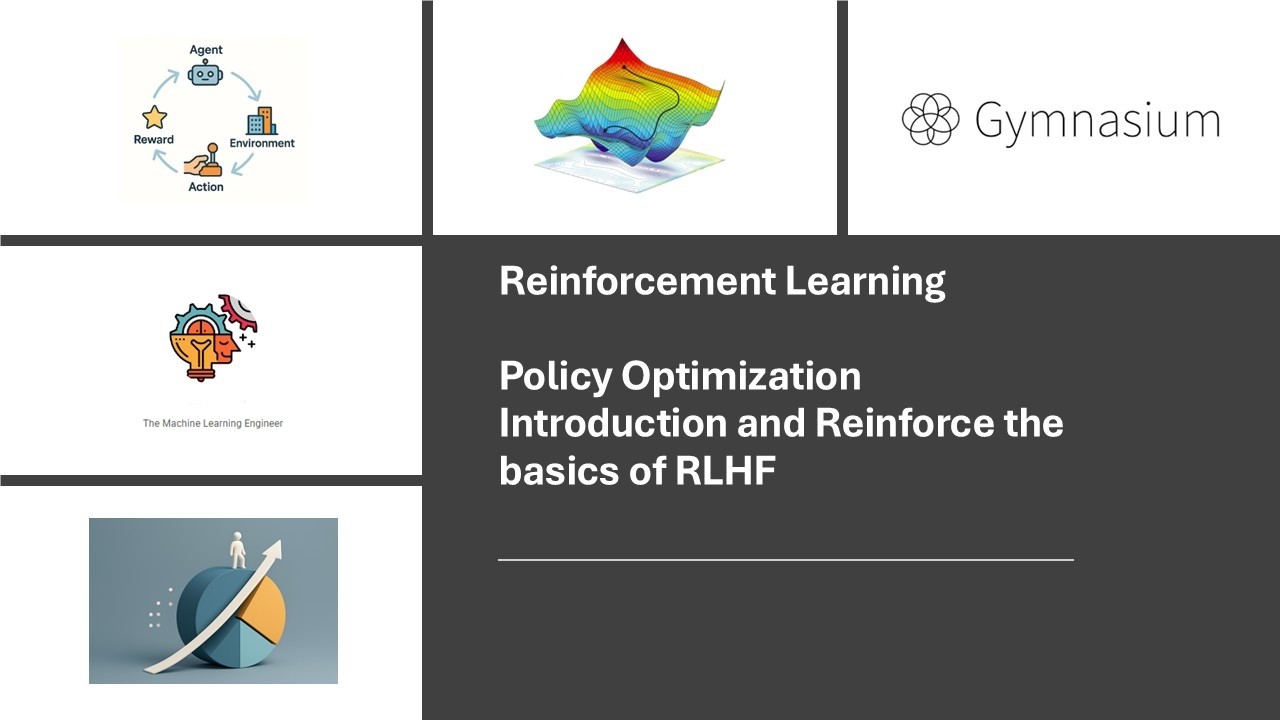
Reinforcement Learning: Policy Optimization Introduction. Reinforce to PPO to RLHF #datascience
Machine-readable: Markdown · JSON API · Site index
Описание видео
In this video, we'll explore RL Policy Optimization — REINFORCE from scratch: math, code, and connection to RLHF. We'll build from the ground up how REINFORCE works — the policy gradient algorithm that forms the basis of PPO and LLM fine-tuning with RLHF.
No prior RL knowledge is required. We'll start with MDP and work our way up to functional code in PyTorch.
**What will you learn?**
▸ What a policy is and why optimize it directly (vs. learning Q-values)
▸ How to model a policy gradient: state, action, reward, path, and discounted return
▸ Why we use stochastic policies and how exploration arises intrinsically
▸ The log-derivative trick — the mathematical insight that makes policy gradients possible without an environment model
▸ The policy gradient theorem and what each term in the central equation means
▸ Value functions: V(s), Q(s,a), and the advantage function A(s,a)
▸ The four variants of the policy gradient and how each reduces variance without changing the estimator
▸ Monte Carlo in REINFORCE: why it is unbiased but noisy, and how to normalize it
▸ The REINFORCE algorithm step by step — with direct mapping to PyTorch code
▸ How the neural network learns the policy episode by episode (Weight evolution)
▸ Implicit Exploration vs. ε-greedy: Why REINFORCE doesn't need manual scheduling
▸ Why policy gradients are the foundation of RLHF and how PPO extends this
**The Repository**
A benchmarking suite for policy optimization algorithms on CartPole-v1. Includes standalone implementations of REINFORCE, A2C, A3C, PPO, and TRPO, a unified orchestrator for comparing all methods, and result aggregation scripts.
📌 Code: [link to repo]
Key files for this session:
- policy_gradient.py — REINFORCE implementation
- policy_gradient_benchmark.py — standalone runner
- run_all_comparison.py — multi-algorithm comparison
- aggregate_results.py — run aggregation
- 03_policy_gradient.md — algorithm reference document
#ReinforcementLearning #DeepLearning #MachineLearning #DistributionalRL #PyTorch #Python
Code:
https://github.com/olonok69/Reinforcement_Learning_Policy_Optimization/blob/main/README.md