Hypothesis tests for one mean: Introduction | Full lecture (Intro Stats)
39:48

Hypothesis tests for one mean: Introduction | Full lecture (Intro Stats)

jbstatistics 23.02.2026 1 039 просмотров 21 лайков

Machine-readable: Markdown · JSON API · Site index

Поделиться Telegram VK Бот
Транскрипт Скачать .md
Анализ с AI
Описание видео
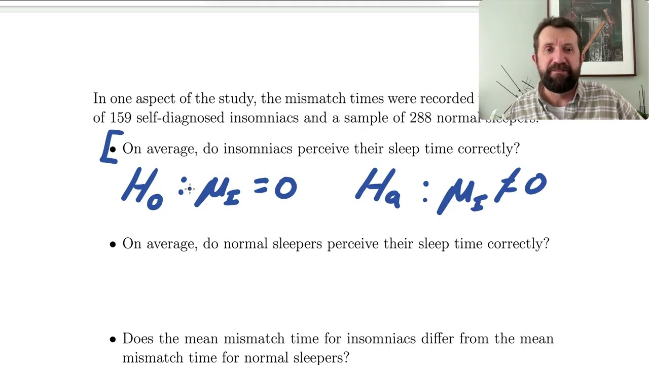
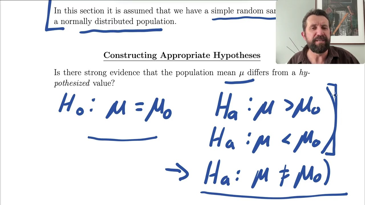
This is a full lecture-style video, discussing tests for a single mean. It is pitched at the level of an applied introductory statistics course at university. I work through the logic of t vs z, motivate the test statistic, and work through an example. This is not a recipe video----the focus is on statistical thinking and why this method works, not simply how to carry out a test. I discuss rejection regions and p-values in the video that follows. Here I continue to work through my lecture outline document, a condensed version of the hypothesis testing chapter from my textbook. Students in my STAT I course at the University of Guelph have these materials. If you're looking for a quick procedural walkthrough, this isn't the right video for you; these lectures are about statistical thinking. I have many shorter videos dedicated to specific topics that may be more appropriate.

Оглавление (8 сегментов)

Segment 1 (00:00 - 05:00)

Hello everybody. Today we are going to continue our discussion of an introduction to hypothesis testing and talk about a specific hypothesis test now and the math behind it and all the details and that is hypothesis tests for the population mean mew. These types of tests are not typically as interesting and formative and used as when we're comparing different groups and trying to see if there's differences between groups or exploring relationships between variables. but they are still important and definitely do help us answer real world questions and are a fairly simple introduction to the specific details behind hypothesis testing. So let's continue on here. We are going to assume at first that we are uh having drawing a simple random sample from a normally distributed population. This is the same assumption we had in a conf confidence interval setting for a single mean. And uh the mathematics behind the hypothesis test very much the same type of thing. we're dealing with the sampling distribution of Xbar in different settings and and related notions. So the math here for the hypothesis test on a single mean uh very much related to the math behind uh confidence intervals and we'll see more on that as we go. The simple random sample part the fact where um you know there's a specific thing what that means I'm not going to get into the specific details of what a simple random sample is here. We've covered that in detail previously, but just big picture-wise, let's keep in mind that if we have biased samples and we're trying to use those to extrapolate out to a population, uh then we're going to be facing problems. So, the sampling design is uh very important in all of this, even though sometimes I might gloss it over in examples because we've got so much uh so much stuff to talk about in the context of hypothesis tests and a lot of it is nuanced and so I'll be talking about all of those details. I might at times kind of gloss over the sampling issues, but they are always always important. How do we get our sample? What sort of biases might be involved if we're trying to extrapolate out to the population of interest? Uh the normally distributed population part like in confidence intervals. This is very important if we're going to use these methods that I'm going to show you today for small sample sizes, but it becomes far less important for larger sample sizes largely due to the central limit theorem. uh and so this the underlying math very similar between confidence intervals and hypothesis tests. So these assumptions and the assumption of a normally distributed population has the same importance here uh as it did in confidence intervals. We'll talk more about that relationship between them a little later on. So constructing appropriate hypothesis here the question is do we have strong evidence that some population mean mew differs from a hypothesized value that is of interest to us for some reason. And we will look at examples of this. It's not just we're making up something to test for kicks. We're only going to carry out a hypothesis test if we have a hypothesis. We wish to test some question about the real world that we're trying to answer. And so we would will test the null hypothesis. Our null hypothesis is going to be no. The population mean does not differ from that hypothesized value. So mu the true well the true mean or population mean I use those two terms interchangeably. If I say population mean or I say true mean it's the same thing. So, mu, which is still representing what it always has, this true mean of our population or of our distribution or what we're investigating, the true mean of your entire population. Um, and that we're going to test the null hypothesis that is in fact is equal to some hypothesized value mu not. So we say that uh and so our null is that hey it the mu is equal to mu not and this is some value that is of interest to us and we'll look at examples of this. Now your alternative essentially is that this is wrong. Your alternative hypothesis is that your null is wrong but it can be wrong in uh a few different ways and we're going to choose one of these uh possible alternative hypotheses. So we're going to pick one of these. One choice, one possible choice is that mu is in fact greater than mu not. And we call that a onesided alternative hypothesis where we're only interested in whether mu is in fact greater than that hypothesized value of mu not. And of course you're going to be able to guess this second one where we're interested in the other direction. Mu is less than mu not. We're interested in seeing whether we have evidence that the true mean is in fact less than mu not. And then uh we have the twosided alternative hypothesis where we have that mu differs from mu not. Now, these are onesided uh alternatives and this

Segment 2 (05:00 - 10:00)

down here is a two-sided alternative and I am of the school of thought that we should be picking this one in the vast majority of cases. If we are interested in a difference in either side, then we should be investigating that with this two-sided alternative. Here's where some of this gets a little bit uh tricky statistically and we can get into arguments about certain aspects of this. But when we say this two-sided alternative in the real world in practical cases in the real world, we are not simply just interested in if there is a difference that is just not the entirety of what we're interested in. This isn't we're testing the null hypothesis that they are equal and then oh we have evidence that they're different. Not just that, we are almost always interested in the direction of the difference. Do we have evidence that mu is greater than mu not? less than mu not? But we're interested in both sides. So this two-sided alternative can be viewed in a way. Don't listen to the pedants here raging in the background. in a way I said as a combination of these two things where we're allowed to see direction here in either direction and this is typically uh what we are interested and we're very often interested in seeing if there's a difference in in either direction. Um, if we take this to the two sample case or when we're trying to test the null hypothesis that two true means are equal or phrased another way that two different groups have the same population mean like a drug and a placebo group, right? We're testing the null hypothesis that those two things uh two true means are equal. Then we're not just looking to see if there's a difference. Oh, there there's a difference. There's a follow-up question there. Which way does the difference lie? you're comparing two drugs, which one is better? Right? So, we're almost always interested in the direction of the difference, not just that a difference exists. This is almost always almost meaningless on its own without the direction saying something about the direction. More on that later. There's some statistical sort of a small statistical issues there in in my view. But we are going to be choosing this as the default the two-sided alternative as the default in the vast majority of things that we do. Uh and then if we are going to pick this one-sided one, one of these if we are interested in only one of the sides. Uh and more details on that later. I discuss this in more details later, but we'll look at that along the way. Okay. So this is what we're interested in. Null hypothesis, mu is equal to some hypothesized value. Alternative that's wrong. We need a test statistic. Now, and recall these important notions that we've discussed in a variety of spots. We're going to have a test statistic. So we have the null hypothesis, alternative hypothesis. Now we're going to construct an appropriate test statistic. And if we're carrying out a hypothesis test for uh the mean of a normally distributed population, it comes down to these two in the same way, the same idea, the same logic here as we had when we were discussing confidence intervals for a single mean. We had these two scenarios. Uh and we discussed these important scenarios here where we had this quantity, right? This quantity here has the standard normal distribution. If we're st sampling from a normally distributed population and this quantity down here has the t distribution with n minus one degrees of freedom. This is very going to be very important because we're going to base our test statistics on this logic. A brief aside here, don't write this down. But just to to be clear here what I'm doing. Side note, important side note really in the grand scheme of things, but it's still a side note. Don't write this down. Okay. When we talked about random variables initially and we had some random variable X, we drew a distinction between the capital X which was represented the random variable and a realized value of X which we put as a lowercase X. This realized value of our random variable X. Then when I talked about the sampling distribution of the sample mean, we had this Xbar capital Xar representing the random variable Xbar and then little Xbar representing a realized value of that random variable. to keep up with this mathematical rigor here, we would need two two of these every time where we'd say the capital T and capital Xar and capital S that is a random variable with this T distribution and then the lowercase version of all of those is a realized value of that random variable. This gets really junky at this point and I'm not going to do it. I am going to have but one formula, not have these two formulas everywhere and which one's this

Segment 3 (10:00 - 15:00)

and why are we doing this and why do we have two and all of this. I think in applied statistics it's just not the way to go. So I'm going to have the one formula for the t. I'm going to have it be based on this notion. And at this point we're going to say that sometimes this thing represents the random variable itself and sometimes it represents a realized value of the random variable. This is the sort of logic that we're going to use in the formulas going forward. So uh we base our statistics uh test statistics on these notions. And remember this is the this very important idea up here that this sigma the true standard deviation right or also known as the population standard deviation a parameter and we almost never know that value in practice. When are we going to know sigma but not know me mu? We're carrying out a test on mu. Implied in that is we don't know the value of mu. How are we going to know the value of sigma? And we can construct situations where conceptually uh but no. So in practice, we're just not going to know sigma. And so in the real world, we're going to be carrying out t tests uh quite often because we don't know sigma. We estimate it with the sample standard deviation s and it's going to lead to a t statistic. Okay, those are important notions for us. Moving down here, we have something very much based on that. So, if we're sampling from a normally distributed population, the appropriate test statistic will depend on whether we know the population standard deviation sigma. And we are not typically going to know the population standard deviation is just not something that arises very often in practice. So we are going to have these still it's still important to know the going through this for reasons I've discussed before and just the notion that the structure of these zed tests is a good thing to know because they do arise in other situations. We zed tests are a real thing in statistics just in this situation we're not typically going to know sigma. That would be a rare case where we'd know sigma and we'd be allowed to use the zed statistic. The more common one situation is that we don't know sigma. We get it based on sample data. And so over here we're going to put s in the formula. And then we have this t statistic. Now we have a very important notion. Where did these come from? These came from these ideas we just talked about. We know this before, right? We we've discussed this before that this quantity uh has the standard normal distribution and this quantity has the t distribution when we're sampling from a normally distributed population. So what do we do? We replace mu with its hypothesized value. That's what's happening in the test statistic. We're replacing mu with its hypothesized value. And okay, but why does that matter? Well, then the null hypothesis is that mu is equal to the hypothesized value mu not. So if we put mu not in there, we get this idea down here. Which means if the null hypothesis is true and that means mu equals mu not right. So if the null hypothesis is true and our assumptions are true like normality uh then this zed statistic here will have the standard normal distribution and this t statistic will have a t distribution with n minus one degrees of freedom. Okay so we're typically going to be using this t statistic over here if we happen to know sigma somehow we'll be using this zed statistic. Now this goes beyond uh this test for one mean. This is an important notion here in the world of statistics and hypothesis testing. What we do is we construct a test statistic that has some known distribution in the event the null hypothesis happens to be true. Like if the null hypothesis is true, this test statistic will have a certain distribution. Then what we're allowed to do is say hey if the null hypothesis is true the value of the test statistic that we get should behave like the value we get will actually be a random sample from that distribution. So if we get an ordinary everyday typical value from that distribution we're not going to have any evidence against the null hypothesis. If we get a really weird value to get from that distribution we're going to have a lot of evidence against the null hypothesis. That's not just here. That's hypothesis testing in general largely. And so this concept here, what I'm talking about extends far beyond here. The big idea, we construct a test statistic that has some known distribution under the null hypothesis. If the null hypothesis is true, get an ordinary value from that distribution, no evidence against the null. Get a really weird value from that distribution, lots of evidence against the null. That's how this works. Okay, so these are our test statistics. We'll

Segment 4 (15:00 - 20:00)

typically be using the t conceivably could be using the zed, but I'm downplaying the zed here in this setting. But zed tests are very important in statistics. They come up a lot in a variety of settings. So it is meaningful, very meaningful for us to uh see these as well. Okay, couple of notes here. The observed value of our t test statistic tells us how many standard errors the value of xbar is from the hypothesized value of mu. Let's just go up up for a second and take a look at this. This recall is our standard error of xbar. That's what that quantity is. Our standard error of xar is s over root n. It's not a fluke that that's there. We are putting in the standard error of xbar. We're taking Xbar, our estim estimator here of of mu, subtracting off the hypothesized value mu not, and then dividing by the standard error of Xbar. And so what that's doing is this. That observed value of the t test statistic tells us how many standard errors the value of xbar is from the hypothesized value of mu. How many standard errors xbar is away from mu not. If that's a lot of standard errors, then that's going to be giving us lots of evidence against the null. And if Xbar is close to mu not in terms of standard errors, then that there's not going to be a lot of evidence uh against the null hypothesis. So this type of test statistic, this form happens a lot. So it goes beyond what we're talking about now. And if you understand this, you're going to understand a lot of what we're doing later. That form happens in a lot of places where this test statistic is going to be our estimator. Here we're saying Xbar. Then we subtract off a hypothesized value that we're interested in for some reason. And then we divide by the standard error of the estimator. And this is going to tell us in all these spots how many standard errors the value of our estimator is uh away from the hypothesized value that we have. So this same logic holds in a lot of test uh testing situations that we have this type of test statistic. Not all sometimes we have very different forms for these things but this is a very common uh form for a test statistic in hypothesis testing. Let's look at a concrete example here. Does the mean amount of cereal in cereal bags differ from the weight stated on the bag. I was interested in this for a variety of reasons and so I have measured weights of food stuffs on a lot of occasions and this particular one on a sale of Sally's sweet wheat bundles at a grocery store. I bought 15 bags from a large selection that were on sale. So I like this cereal. I eat a lot of cereal. I'm a fan of cereal. Uh so I thought, hey, this is a good deal on these bags. I will eat them. And plus I can do some weighing for statistics examples. So, uh, I got 15 bags. And I tried to do it as sort of randomly as I could. You know, human being doing that stuff. You can't do it purely randomly. But I just tried I wasn't cherry-picking bags, holding them in a hand, seeing if anything was heavier than another. I was trying my best to randomly pick from a large number of bags that were on sale that day. And so, really, I think it's reasonable to think that the bags I got could be viewed as a random sample of the bags on sale that day at the grocery store. Uh, and we can talk about that a little bit more. The sampling design, how far out we'd go. We talked about this a little bit when we talked confidence intervals. I'm going to gloss over that a little bit today because we're focusing on hypothesis testing. But the sampling design once again is always important. Each of the bags had a stated weight of 368 g. So we might be interested in testing the null hypothesis and I was that mu is equal to 368. I don't really know and didn't know at the time what typically happens with with food items and how much they actually put in there when they state that. A pretty good suspicion that they tend to give us at least that amount. But a reasonable thing to look at here is saying, "Hey, are we getting when we buy these things, are we getting more bang for our buck or less than the company's stating? " Certainly a reasonable thing to check out and companies in the past have been found to be systematically underfilling things at times. So that is not all that common, but it has happened. So we might want to test this null hypothesis. Now, we would have the choice right at this point. I could pick the alternative that mu is greater than 368 if I'm only interested in whether it's greater than or mu is less than 368 if I'm only interested in if it's less than 368. But really I'm interested in a difference in either direction here. I would care if it's on both sides. I care if it's greater. That's kind of nice to know I'm getting more than I than they're they're stating on average. Uh and I certainly care if I'm getting less than they're stating on average. So I think an appropriate alternative here

Segment 5 (20:00 - 25:00)

would be that the two-sided that mu is not equal to 368 because then we're able to see a difference in either direction and I'm interested in direction. So this is what I would intend to to investigate when I was buying these serial bags before I even took the measurements. I was intending on on checking this out and testing this null hypothesis. So again this is mu is the true mean serial weight in bags of this type or the population and the hypothesized value is 368. This is our mu not in this case. Right? Uh and we could talk go on and on about in details about what precisely mu means here with the sampling design and how far out we can extrapolate and what the target population is. I'm going to leave that a bit to the aside here. A simple version, a simple quite reasonable one would be saying um that our population would be all bags of cereal uh on sale that day at that store. We probably do want to say something beyond that, but that gets a little bit trickier and trickier because you technically only sampled from that store that day. We'll talk about more about these sorts of things later, but the sampling design always important. Glossing it over a little bit here. This is what we got. This is what I got. So, I went through and I got those the serial weights. I did this very carefully. I, you know, shook it all out, right? I was very careful about getting this as as accurately as I could down to the gram. Anyway, um, and so these are the 15 weights that I got. Uh, my sample mean 374. 47. My sample standard deviation is 2. 825 g. So this is overall here uh a little bit uh bigger than that 368. Keep in mind and this is important and many textbooks completely botch this idea like they really do that. Keep in mind we do not use this to inform our hypotheses up here. These hypotheses when you're creating hypotheses you should always remember you should be able to create those before ever looking at your data. This data itself should not influence these hypotheses. You come up with those based on this research question of interest, not what you see in the sample. You use your sample data and form your hypothesis, you're just screwing up the math completely. Just not okay. So, I came up with the hypothesis based on the setting and what I was interested in and then the sample values. I got this. And does this sample yield strong evidence that the true mean weight of these sweet bandal uh of cereal in these types of bag differs from that stated uh value of 368 grams? Pretty natural question. 374 was a little higher, right? Looking at that. Okay. On average, we're getting a little six grams more than stated on the on the bag. Uh but it does this sample provide strong evidence that we are in fact truly uh getting more than the 368 on average? Um or and let let's take a look. Let's first have a look at this box plot over here. This is addressing the big picture question of what we're investigating. So I have a jittered box plot. So this is a regular box plot with the data points in here. So these are the values. The vertical axis is still values of the serial weights along the way. Uh and just giving us we can see the actual serial weight values in there. Helps us to visualize things. And I've also put just a little red dash and I like to put in my box plots a little red dash indicating where the sample mean is. So that's the sample mean. And I put down here this 368 which was our hypothesized value of mew. That's mu. Well, right away visually looks like we have a lot of evidence that we are in fact getting more than that than that hypothesized value of 368. The sample mean was up here. Certain bit of variability. Of course, they don't put exactly the same amount of weight in each bag of cereal, but just visually gut feel looking at this. that difference between our sample mean and our hypothesized mean. The fact that all of these values are up here, it looks like we have a lot of evidence that the true mean is in fact greater than this hypothesized mean. Looks like that to my eyes certainly. But we're going to see what the hypothesis test has to say on that. Now, we need to check out normality because we have a normality assumption here. And what I have uh done uh is I have these plots. So these are um uh my little plots. You don't see these elsewhere really and maybe somebody has them somewhere. I don't know. But if they do independently discovered so I do the I really like having these plots just like this the JB

Segment 6 (25:00 - 30:00)

plots like this. We have box plots jittered box plots. We can see the serial values. sample mean. We've got the hypothesized mean. kind of visually o overall have a pretty good assessment of the evidence against the null hypothesis but we're investigating the the normality assumption now and we typically do that through normal quantile plots but what help us might help us see things a little bit better is that I have this box plot on the same uh vertical axis as the normal quantile plot so these points map over to the normal quantile plot like so this is the same axis as over here so these are mapping over here. What do we see? Well, we got a couple of bigger values here and here. Uh, other than that, looking pretty good, right? Looking pretty good. I would say we have, you know, one or two mild outliers. You can think of those as mild outliers perhaps. And our sample size is fairly small at 15. So, the normality assumption is quite important. We do have a couple of mild outliers. In an ideal world, we would love it if we didn't. Outliers are an enemy of the T procedure. Outliers and skewess T procedures don't like that. Uh, and we do have something that is a bit of an outlier here. I don't think that's a huge deal here. I think I think it's okay. I think, oh, all right, we got a little bit of an outlier. Maybe that has impact. Maybe we could analyze that in more detail and see what influence it has on our uh test statistics and these sorts of things. Um, but overall, I think it's okay. I think it's reasonable to say that this is approximately normal, roughly normal, and that we can go ahead with the uh t test statistic. It's going to be a t test and not a zed test because we don't know sigma. I don't know the true standard deviation of the fill of the cereal in these bags. I don't know the population standard deviation. This is not known. So when we go up here, we're calculating this. This is based on these 15 bags, which means it's a sample standard deviation, which means I can't use the zed test. It's got to be a t test. So, we're going to go ahead now and calculate the test statistic. So, I put this in here at first because remember again, this form is really common in other things that we do. And I want to remind you of that. Like that's our estimator there, our xbar. This is our hypothesized value of mu. So our estimator of mu minus our hypothesized value of mu and then we divide by the standard error of the estimator. This is a very common type of test statistic that we use in hypothesis testing. It boils down to this. Our standard error of x bar is s over root n. And so we've got this. We calculate the values. Carry many decimal places. Okay. I I rounded here to to a couple right but they carry many decimal places throughout the calculations and we get 8. 87. So 8. 8 87 is the value of our test t test statistic. And we could say that the sample mean xbar is 8. 87 standard errors above the hypothesized value mu not. The sample mean xbar is 8. 87. The value of the sample mean xbar is 8. Let's see what that looks like in terms of distribution. N was 15. So we have our degrees of freedom in one sample problems. It'll change for other problems but for right now for this type of problem n minus one 15 -1 we have 14 degrees of freedom. So what I have done here is plotted a t probability density function with 14 degrees of freedom. That's what that is If the null hypothesis is true, this is the distribution of our t test statistic. The assumptions also need to be true, normality, etc. But if the null hypothesis is true, then our test statistic has this distribution and the value of the test statistic will then be a random sample plucked from this distribution. Our value is out here at 8. 8. 87 way out in the right tail, right? That value is tail. Had we gotten a value down here closer to zero, like a typical value to get from this distribution 72 minus 1. 14, something like that, just sort of closer to zero. We would have said, okay, we don't really have any evidence against the null hypothesis. and we'd just say, "Ah, the data would be consistent with the null hypothesis had we gotten a value down here somewhere. " But we did not. We got a value way out in the right tail, 8. 87.

Segment 7 (30:00 - 35:00)

This is a highly unusual value to get if the null hypothesis is in fact true. That's way out in the right tail. So this is extremely unlikely value to get if the null hypothesis is true. So we are going to say we have very strong evidence against the null hypothesis and in favor of the alternative hypothesis. So our value out here very large very high way out in the right tail. Remember that shouldn't be too surprising given what we saw up here. This this sort of gives us that vibe right just visually and then when we go down here and actually crunch the numbers we are way out in the right tail. So just based on this and we'll shore these ideas up about specifically how far out in the right tail matters etc. But just overall thinking about this like logical humans we are way out in the right tail. If the null hypothesis is true the value we get should just be a random sample from this distribution. And this does not at all look like a value that was randomly sampled from this distribution. It is way out here. So we have very strong evidence against the null hypothesis that the true mean is equal to 368. Uh and so we have very strong evidence in favor of the alternative hypothesis that the true mean differs from 368 and our population g. Now again, in the real world, direction is important. There's a huge difference to a consumer like me between us getting more bang for our buck in this from the cereal on average than what they're stating and getting less. If I'm getting more than that than what they're saying, I'm cool with that. If I'm getting less than what they're saying, I am not cool with that. So there's a direction is important here as it essentially always is in hypothesis testing even when we're using a two-sided alternative. So we could say we can say that there is very strong evidence that the true mean weight of cereal in bags of this type. Specifically what we mean by bags of this type is open to debate here. The true mean weight of cereal in bags of this type or the population differs from 368 gram. But we can also say more than that. The sample mean Xbar was 8. 8 standard 8. 87 standard errors greater than the hypothesized mean. So we have very strong evidence that the true mean is in fact greater than the hypothesized mean of 368 g. So even when we're using a two-sided alternative, in almost all cases, we are very interested in the direction of the difference. We get into some uh subtle statistical issues when doing this. Uh but they those issues are very small relative to just saying something essentially silly like oh all we can say is that it differs from 368. The real world we want to know where the the difference lies. the direction of the difference. So there very strong evidence just as logical humans looking at this that the true mean weight of cereal and bags of this type is in fact greater than the stated weight of 368. Now in the real world we do this in software. So let's see what that looks like in R. We'd have similar things if we did this in other software programs or status or variety of things we could use Excel. But if we did a t test t. est this I am inputting my vector of 15 serial weights in there. And then here I have to tell r uh what we're testing. R doesn't know what we're testing just based on the numbers. Right? So this is our terminology for uh we are testing the null hypothesis that mu is equal to 368. [snorts] We can also tell r what the alternative hypothesis is. But it takes as a default the two-sided alternative because it says this here alternative hypothesis the true mean is not equal to 368. Uh so it has that as a default but you can change your alternative a with an option here. This was our test statistic. This is what we got. So I rounded a little bit when we got our 8. 87 up here but our is getting that. So that's just just rounding error on our part. Uh that is the value of the test statistic 14 degrees of freedom. Always useful to check your degrees of freedom in your output. Sometimes you screw up and you give it wrong data. You ask it for the wrong thing. Always useful to check your degrees of freedom. So that just a little double check here just to see we do have 14 degrees of freedom. That is what we were thinking. Okay, reasonable. This p value. We'll talk about this in great detail soon. And don't worry about it too much. It's a measure of how far

Segment 8 (35:00 - 39:00)

out in the tail you are. Short version, right? But it's very detailed and we'll talk more about that in detail. So don't worry about this p value for now. This confidence interval, we did this before. That's a confidence interval for mu for the the true mean weight in in bags of this type. So this uh this mu uh the confidence interval for mu. We've done this before. We had a 95% confidence interval mu from mu of 372. 9 to 376. 0. Now you might notice that 368 is not in that interval. And so just based on this interval, had we not done this hypothesis test, if I just looked at this interval, I'm 95% confident that the true mean lies between those two values. And 368 is quite a bit to the left here. It's not in that interval. This whole entire interval is well to the right of 368. Just based on a little bit of logic there, we we could say based on the interval that there's quite a bit of evidence that the true mean is greater than 368. But we went through this formal hypothesis test procedure because we had that very that point of interest that 368 that we were interested in. Uh and so when we were interested in something like that, we really should carry out the formal hypothesis test. One thing that does for us is it allows us to give a measure of the strength of the evidence against the null hypothesis that we'll talk about when we talk about the p value a little bit later on. But this confidence interval, which we've done before, just looking at that would give us a pretty good idea of what's going to happen in the test. And in fact, there's a very direct relationship between hypothesis tests and confidence intervals. But we're going to talk about that a little bit more detail later when we talk about a few more concepts because the language has to be just right. Okay. So that this is this is our output. We're going to be using this quite often in things like this and coming back to that. Now a very natural question here though if we go back up here. A very natural question is we say okay well we were way out in the tail here. tail. So sure just as logical humans we're saying we're way out in this tail. We're almost nine standard errors greater uh than the hypothesized mean. There's a lot of evidence against the null. This does not look like a value we would get if we were just randomly plucking from this distribution. We might you can get anything any finite value, right? But this looks like it'd be pretty unlikely to get something this far out in this uh in this tail. That just it just does not look very like likely. So, as logical humans, we're saying we have a lot of evidence against the null. a lot of evidence that the true mean uh weight of cereal in bags of this type is in fact greater than 368. And like I said, if we got a value down here, we would say no, we we don't have a lot of evidence uh against the null hypothesis. A value down here sort of closer to zero, you know, minus. 87 1. 16, we' say, oh, these are normal everyday values to get from this t distribution. So the data is consistent with the null hypothesis being true. If we got something down here, maybe the null is true, maybe it's not true. This sort of this sort of idea, but we wouldn't have any evidence against it if we h got a value down here, a route close to zero. But then the natural question, where do you draw the line? Okay, so if we got something here, we don't wouldn't have a lot of evidence against the null. We got something way the heck out here, we do have a lot of evidence against the null. What if we got six? Yeah, that'd be a lot of effort still. But how about if we get something, you know, not quite so clear? How about if we got a value around two or 1. 8 or this sort of idea? How far out in the tale do we have to be in order to say that we have strong evidence against the null hypothesis? Very natural question at this point. And there's a fair bit to it. So we have a couple of approaches at this point. One is the rejection region approach where we make a fixed rule and we see if our test statistic falls in a rejection region. Another is a p the p value approach where we give a measure of how far out in the tail that test statistic is. And those are important things in the world of statistics. A little bit nuanced, a lot nuanced. So we're going to talk about those issues in another video when I talk about rejection regions and p values. That's coming up soon. I'll see you then.

Другие видео автора — jbstatistics

Ctrl+V

Экстракт Знаний в Telegram

Экстракты и дистилляты из лучших YouTube-каналов — сразу после публикации.

Подписаться

Дайджест Экстрактов

Лучшие методички за неделю — каждый понедельник