Before and After - Fixing a Real Slow Postgres Query

This query runs in about 5 minutes. It's not that long. It's not that complicated, but if this was sitting inside a production application, that run time is a problem. In this video, I want to show you the exact steps I take to investigate a slow query like this, find the cause and fix it. We'll look at the execution plan, work out what's going wrong, and make changes based on evidence rather than guessing. I'll also use an AI tool to analyze the query and compare what it finds to what I find myself. And if you want to improve the performance of your queries, I've put together a free SQL performance checklist. You can grab it from the link in the description. Before we change anything, let's understand what this query is actually doing. Here is the query we are working with. This is running on the Chinook database, which is a sample database for a fictional music store. I've added extra rows to the tables to make the performance problem more visible. So, what does this query do? It joins to the invoice line table to itself. We're looking for pairs of invoice lines for the same track where the unit price of those two lines was within $1 of each other. Then we count how many times that happened per track and return the top 50. That's a legitimate question to ask about the data. But the way it's written creates a real performance problem. Why? Let's look at the execution plan and find out. This is the first thing I do

with any slow query. Before I rewrite it or add an index, I read the execution plan. The execution plan shows you the steps the database takes to run the query. Think of it as the database showing its work. In DataGrip, I'll right-click on the query and select explain plan. A panel appears at the bottom. This is done differently in each SQL editor, but there usually is a button on the toolbar or in the menu. Now, this looks like a lot, but you won't need to understand every single step. Start with the basics. The most indented steps are the starting points. The database works from the inside out. We can see the process starts with reading data from the track table using the full scan step here. Then data is read from the invoice line table in the entry above and joined again using this hash join step. Then the database reads from the invoice line table again and combines the results. There are many other steps performed as we work our way up the list until we get to the select at the top. We can see the overall cost, which is 7780779. That's our baseline number, about 7. 7 million. The cost is a measure of the effort the database takes. It's not a unit of time. Now, we can look at the individual steps and see where the cost is concentrated. There are a couple of things I want to point out here. One is this step that relates to the self-join on the invoice line. You can see that two branches of the plan are reading from the same table. That's our self-join in action. The other thing is the cost of this hash join compared to everything else. It's taking up a significant portion of the total query cost. Here it says the cost is 7362806. This cost is for this step and everything underneath it. Even if we subtract this 45,000 step and this 42,000 step, we still have a cost of about 7. 2 million, which is almost all of the cost of the query. The third thing to notice is that there is no index being used here for this join condition. It says full scan, meaning the entire table is read. We'll come back to why in a moment. Now, before we make any changes, I want to save this execution plan as our baseline. This is important. If you don't measure before you start, you have no way to tell whether your changes actually helped. I'll save this as a screenshot as we can add it to our AI tool later in the video. We could save it as a file or copy the text, but screenshots are good enough for now. Good. We have our baseline. Now, let's work out what's causing the problem. The first issue is the self-join on invoice line. A self-join is where you join a table to itself. In this query, we have two aliases for the same table, IL1 and IL2, and we're matching rows from each. The first part of the join is fine. We're matching rows with the same track ID, and the condition IL1. InvoiceLineId is less than InvoiceLineId from IL2 makes sure we only get each pair once and not twice. But the problem is scale. If there are a large number of invoice lines for a given track, the database has to compare every qualifying row against every other qualifying row for that track. As the table grows, the number of comparisons grows much faster than the number of rows. On a small table, you won't notice this. On a large table, it becomes a problem quickly. That's what we're seeing here. The invoice line table has a lot of rows, and this join is expensive because of it.

The second issue is this line here, which uses the ABS function. ABS stands for absolute, and it's a way of converting a positive or negative number to its positive version. So, if we are subtracting one price from another and the value is negative, then it is converted to a positive number. This is done so it can be checked that it is less than one. This is what we call a non-sargable condition. That term sounds complicated, but the idea is straightforward. Sargable stands for search argument able. A condition is sargable if it the database can use an index to resolve it. A condition is non-sargable if it can't. When you wrap a column in a function, in this case wrapping unit price inside ABS, the database has to calculate the result for every row before it can filter. It can't look everything up. The index on that column, if one exists, is bypassed entirely. Compare that to a range condition like this. Both of these say exactly the same thing. Any pair where the unit prices are within $1 of each other. But the second version expresses it as a range on the column directly, which gives the database a better chance of using the index. This is one of the most common performance patterns I see. The query is logically correct. The result is right, but the way the condition is written silently prevents the index being used, and the execution plan is often the only thing that makes it visible. Let's make this change and see what happens. We'll update this join condition. We'll remove the ABS call and replace it with these two range conditions. The unit price of IL2 has to be greater than or equal to IL1. UnitPrice - 1 and less + 1. Before we go ahead with this query, there's something to check first. We need to confirm if the results are the same. It's easy to introduce a subtle mistake when rewriting a condition, so I always check this. The row count matches. A few spot checks on the values look consistent. We can see the run time is 6 minutes and 50 seconds, which is quite a bit slower than the original query. Let's run the execution plan on the version of the query now. We can see the plan here. The cost has changed. The old cost, the original cost was 7. 7 million, and the new cost is 8. 2 million. So, this has actually made things worse. The range condition should have given the database more options for how to access the data compared to that function wrapped version. Each of the tables are still being accessed by this full scan method, so it looks like any indexes are also not being used. That said, there may be more we can do.

Let's look at whether an index would help here. Let's check whether there are useful indexes on the invoice line table already. I'll open the object explorer here, expand the table, and look at indexes. We can see that there's an index on the invoice line ID, which makes sense as the primary key. There's also one on invoice ID and track ID, but there doesn't seem to be an index on unit price. This is one of the columns being used in our join conditions. Let's try adding an index on unit price to help the self-join. One of the conditions in our join is matching rows on the unit price, so an index on that column could reduce the work the database needs to do. We run this and the index is created. Let's see the execution plan. The index has not been picked up here. This is interesting. It could be because the database is using a few other criteria to perform a match, so using the unit price isn't enough to filter the data so the index can be used. Let's see what else we can try. One other technique we can try is a covering index. A covering index is where the index includes all of the columns that the query needs from that table. If the database can get everything it needs from the index without going back to the table itself, it can be noticeably faster. Let's look at what columns from the invoice line are actually used in this query. We use invoice line ID, track ID, and unit price. We can create an index on track ID, since that's our most selective join column, and include the other columns. Let's check the plan. We can see the covering index is not being used here. The cost is the same. So, this hasn't worked either. This is a good illustration of something worth understanding about indexes. They don't always give you the gains you expect. The database makes decisions based on the data, the query structure, and the available indexes, and sometimes the best option still involves a lot of work. So, what's our latest run time? The original run time was 5 minutes 23, and we ran it again after changing this criteria and got about 6 minutes and something.

something. Now, let's see what an AI tool makes of this query. I'll use Microsoft Copilot here. If you're working at an organization that uses Microsoft tools, you may have access to an enterprise version, which keeps your data within your organization. That's worth checking before you use any AI tool with your company's code or data. I'll use a prompt that asks the tool to analyze the query and execution plan and suggest improvements. The prompt I'm using here is available as a free download. The link is in the description. Let's run this and see what it comes back with. The first thing it's flagged is the self join on invoice line. It's noted that this is scanning a large table twice and that the join condition is expensive. That matches what we found. It mentioned something about sequential scans on the invoice line and track. It also mentions no indexes are used, which is similar to what we found as well. We tried to create a couple of indexes, but didn't have much luck. The third point is around no indexes used for price filtering. We changed our criteria on the unit price here because we found that the sargable condition with the ABS function was not really helping. So, even though we did this, the indexes were not being used. There is a fourth point here about double aggregation and sorting. It says it performs an aggregation, then sort, then aggregate, then sort. It says these operations are redundant and there is an impact to CPU and memory usage. So, what are the recommendations here? This one is interesting. It says the top recommendation is nothing to do with indexes. It says to actually rewrite the query to reduce the join explosion. We kind of noticed that this in our original query was the most expensive step where it tried to join the two invoice line tables together. It says here, instead of joining invoice line to itself, consider using a window function or pre-aggregating. The pre-aggregation means that we're actually using a select statement to come up with the data we need first at the right level and then joining other tables to that. And it mentions here that this will isolate the heavy join and lets you optimize it separately. That's an interesting approach, so something we should definitely try. Let's see what else we have. We have some indexes here on a couple of the columns, which we can also try, and also a functional index if this ABS function is actually used. There's also an option to update the statistics as well, which might impact the row counts, but it says this is less likely. We have a prioritized list of fixes here, which we have an index and a query rewrite at the top here.

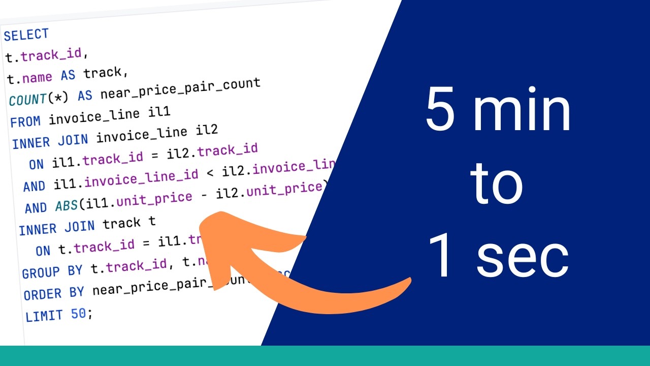
Let's try this suggestion of the rewritten query on our database. We can copy the query here and paste it into our editor. Before we run the query, let's understand this. It uses a CTE, which is the with clause, to select some invoice line data. It still has the self join to the invoice line table. It also uses the ABS function, which we commented out from our earlier query, but Copilot has added it back in. In the CTE, it finds the track ID and the count of pairs with the price near another invoice line. Then, in the main query, it joins to the track table to get the track data. It seems to match what we want to do. So, let's run the query. After a while, the query finishes. The results look the same at first glance. However, it ran pretty slowly. We can see the runtime here was 5 minutes and 44 seconds. This is not much different to the original. Let's see the execution plan. Not much has changed with the execution plan. We can see some of the ordering of the data retrieval steps have changed. It has these two invoice line items here and then the index scan is done on the track table later in the process. The overall cost is 7,777,080 or 7. 7 million. I think the AI tool was heading in the right direction, but there's probably another way we can do this. Let's think about the query. The performance is slow because of the large number of invoice line records that need to be compared. How about we try to reduce the number of invoice line items that are compared? Instead of comparing each row, we find the number of tracks sold at each price and compare those numbers. So, we can perform some aggregation for tracks and unit prices and compare that data. This may result in less data being compared. We'll start with this with clause to calculate the result set of tracks and prices. Inside this, we select the track ID, the unit price, and the number of records of tracks at that price. We then group by these two fields. Then, we have another common table expression. In this query, we want to get the track IDs and the number of invoice lines where the price is within one. We select from the price count CTE, which we defined earlier. We select from it twice because we want to see the matching tracks. We join on similar criteria as the original query, on the track ID and on the unit price. Now, how do we find the number of invoice lines that meet this criteria? To do this, we use this case statement. In the case statement, we check if the unit price matches between both tables. If it does, we add this calculation here. The count of records multiplied by minus one, then divide by two. This is a mathematical formula to find the combinations of two items, excluding the combinations that exactly match. So, if there is a single track and a price of 199 and a count of five, then the calculation will return 10 because there are 10 combinations and not 25. Now that we've done this calculation, we can select the final columns we need. We select the track ID, the name of the track, and the sum of the near price pair count. We join the track table to our pairs CTE, order our results, and limit it to 50. Our query is now ready. Let's run it. We run this and it completes almost instantly. That's a big improvement. We'll have to check the results are correct, but it's fast. On the output tab, we can see the runtime is 1 second and 429 milliseconds. Let's see the results. The results look okay. However, let's compare them to the original. I'll select these results and copy them. Then, I'll paste them into this spreadsheet here. I prepared this earlier and it shows the original results on the left. This formula here compares the two result sets and we can see that all rows are matching. This is good to see. So, the results match and the query is faster. We can see here it looks quite different. At the bottom, it gets some data from the track table and then creates the price counts object. This is referred to twice. An important thing to note here is the row count. There is an estimate of 7,000 rows here and when it is combined, it's about 27,000. This is much less than the original. Further up the execution plan, the invoice line table is read and it's only read once. We can see some more operations are done and the overall cost is about 60,000. This is a massive improvement to the 7. 7 million of the original query. The AI analysis helped us a little with this rewrite, but the version it provided didn't improve performance. It helped to point us in the right direction, though. So, what did we do with this query? We started with a slow query. We ran the execution plan and found two things: a self join on large table and a non-sargable condition using the ABS function. We fixed the non-sargable condition by rewriting it as a range condition directly using the unit price column. That gave the database the ability to use indexes where it couldn't before. We added a couple of different indexes to help the join, but they both had no impact on the execution plan or the query runtime. We also compared our analysis to an AI tool and found it identified the same core issues: the self join cost and the non-sargable condition. It also suggested a query rewrite as it understood the logic we were trying to accomplish and found a different way. This rewrite didn't help the runtime, but it pointed us in the right direction. We made another rewrite, which improved the runtime drastically. The final runtime is about 1 second, which is compared to almost 6 minutes at the start. There are a few things to take away from this. The first is about non-sargable conditions. Anytime you wrap a column in a function inside a join or where clause, you should check whether an equivalent condition exists that doesn't require the function. It's not always possible, but when it is, it's worth doing. The second is about self joins. They can be legitimate, but on large tables, they are expensive by nature. Sometimes there's a different way to express the logic with a window function, for example, that avoids the cost of comparing every row against every other row. And the third thing is about the process itself. Baseline first, read the plan, form a hypothesis, make one change, measure, and then repeat. That process works regardless of the query, the database, or the tool you're using. And the AI analysis is a useful part of that, but it's one input, not a replacement for understanding what the plan is telling you. If you want the exact AI prompt I used in this video, it's available at the link in the description. If you found this video useful, you'll want to watch this video next, where I do the same kind of walk-through on a slow SQL Server query and compare my findings against what an AI tool picks up, including one thing that AI found that I missed. Thanks for watching.