Why “probability of 0” does not mean “impossible” | Probabilities of probabilities, part 2
10:00

Why “probability of 0” does not mean “impossible” | Probabilities of probabilities, part 2

3Blue1Brown 12.04.2020 3 300 355 просмотров 83 373 лайков

Machine-readable: Markdown · JSON API · Site index
Поделиться Telegram VK Бот
Транскрипт Скачать .md
Анализ с AI
Описание видео
An introduction to probability density functions Help fund future projects: https://www.patreon.com/3blue1brown An equally valuable form of support is to simply share some of the videos. Special thanks to these supporters: http://3b1b.co/thanks Curious about measure theory? This does require some background in real analysis, but if you want to dig in, here is a textbook by the always-great Terence Tao. https://terrytao.files.wordpress.com/2012/12/gsm-126-tao5-measure-book.pdf Also, for the real analysis buffs among you, there was one statement I made in this video that is a rather nice puzzle. Namely, if the probabilities for each value in a given range (of the real number line) are all non-zero, no matter how small, their sum will be infinite. This isn't immediately obvious, given that you can have convergent sums of countable infinitely many values, but if you're up for it see if you can prove that the sum of any uncountable infinite collection of positive values must blow up to infinity. Thanks to these viewers for their contributions to translations Hebrew: Omer Tuchfeld ------------------ These animations are largely made using manim, a scrappy open source python library: https://github.com/3b1b/manim If you want to check it out, I feel compelled to warn you that it's not the most well-documented tool, and it has many other quirks you might expect in a library someone wrote with only their own use in mind. Music by Vincent Rubinetti. Download the music on Bandcamp: https://vincerubinetti.bandcamp.com/album/the-music-of-3blue1brown Stream the music on Spotify: https://open.spotify.com/album/1dVyjwS8FBqXhRunaG5W5u If you want to contribute translated subtitles or to help review those that have already been made by others and need approval, you can click the gear icon in the video and go to subtitles/cc, then "add subtitles/cc". I really appreciate those who do this, as it helps make the lessons accessible to more people. ------------------ 3blue1brown is a channel about animating math, in all senses of the word animate. And you know the drill with YouTube, if you want to stay posted on new videos, subscribe: http://3b1b.co/subscribe Various social media stuffs: Website: https://www.3blue1brown.com Twitter: https://twitter.com/3blue1brown Reddit: https://www.reddit.com/r/3blue1brown Instagram: https://www.instagram.com/3blue1brown_animations/ Patreon: https://patreon.com/3blue1brown Facebook: https://www.facebook.com/3blue1brown

Оглавление (5 сегментов)

<Untitled Chapter 1>

Imagine you have a weighted coin, so the probability of flipping heads might not be 50-50 exactly. It could be 20%, or maybe 90%, or 0%, or 31. 41592%. The point is that you just don't know. But imagine that you flip this coin 10 different times, and 7 of those times it comes up heads. Do you think that the underlying weight of this coin is such that each flip has a 70% chance of coming up heads? If I were to ask you, hey, what's the probability that the true probability of flipping heads is 0. 7, what would you say? This is a pretty weird question, and for two reasons. First of all, it's asking about a probability of a probability, as in the value we don't know is itself some kind of long-run frequency for a random event, which frankly is hard to think about. But the more pressing weirdness comes from asking about probabilities in the setting of continuous values. Let's give this unknown probability of flipping heads some kind of name, like h. Keep in mind that h could be any real number from 0 up to 1, ranging from a coin that always flips tails up to one that always flips heads and everything in between. So if I ask, hey, what's the probability that h is precisely 0. 7, as opposed to, say, 0. 7000001, or any other nearby value, well, there's going to be a strong possibility for paradox if we're not careful. It feels like no matter how small the answer to this question, it just wouldn't be small enough. If every specific value within some range, all uncountably infinitely many of them, has a non-zero probability, well, even if that probability was minuscule, adding them all up to get the total probability of any one of these values will blow up to infinity. On the other hand though, if all of these probabilities are 0, aside from the fact that now gives you no useful information about the coin, the total sum of those probabilities would be 0, when it should be 1. After all, this weight of the coin h is something, so the probability of it being any one of these values should add up to 1. So if these values can't all be non-zero, and they can't all be 0, what do you do? Where we're going with this, by the way, is that I'd like to talk about the very practical question of using data to create meaningful answers to these sorts of probabilities questions. But for this video, let's take a moment to appreciate how to work with

Probabilities over Continuous Values

probabilities over continuous values, and resolve this apparent paradox. The key is not to focus on individual values, but ranges of values. For example, we might make these buckets to represent the probability that h is between, say, 0. 8 and 0. 85. Also, and this is more important than it might seem, rather than thinking of the height of each of these bars as representing the probability, think of the area of each one as representing that probability. Where exactly those areas come from is something that we'll answer later. For right now, just know that in principle, there's some answer to the probability of h sitting inside one of these ranges. Our task right now is to take the answers to these very coarse-grained questions, and to get a more exact understanding of the distribution at the level of each individual input. The natural thing to do would be consider finer and finer buckets. And when you do, the smaller probability of falling into any one of them is accounted for in the thinner width of each of these bars, while the heights are going to stay roughly the same. That's important, because it means that as you take this process to the limit, you approach some kind of smooth curve. So even though all of the individual probabilities of falling into any one particular bucket will approach zero, the overall shape of the distribution is preserved, and even refined in this limit. If, on the other hand, we had let the heights of the bars represent probabilities, everything would have gone to zero. So in the limit, we would have just had a flat line giving no information about the overall shape of the distribution. So, wonderful. Letting area represent probability helps solve this problem. But let me ask you, if the y-axis no longer represents probability, what exactly are the units here? Since probability sits in the area of these bars, or width times height, the height represents a kind of probability per unit in the x-direction, what's known in the business as a probability density.

Probability Density

The other thing to keep in mind is that the total area of all these bars has to equal one at every level of the process. That's something that has to be true for any valid probability distribution. The idea of probability density is actually really clever when you step back to think about it. As you take things to the limit, even if there's all sorts of paradoxes associated with assigning a probability to each of these uncountably infinitely many values of h between 0 and 1, there's no problem if we associate a probability density to each one of them, giving what's known as a probability density function, or PDF for short. Anytime you see a PDF in the wild, the way to interpret it is that the probability of your random variable lying between two values equals the area under this curve between those values. So, for example, what's the probability of getting any one very specific number, like 0. 7? Well, the area of an infinitely thin slice is 0, so it's 0. What's the probability of all of them put together? Well, the area under the full curve is 1. You see? Paradox sidestepped. And the way that it's been sidestepped is a bit subtle. In normal, finite settings, like rolling a die or drawing a card, the probability that a random value falls into a given collection of possibilities is simply the sum of the probabilities of being any one of them. This feels very intuitive. It's even true in a countably infinite context. But to deal with the continuum, the rules themselves have shifted. The probability of falling into a range of values is no longer the sum of the probabilities of each individual value. Instead, probabilities associated with ranges are the fundamental primitive objects, and the only sense in which it's meaningful to talk about an individual value here is to think of it as a range of width 0. If the idea of the rules changing between a finite setting and a continuous one feels unsettling, well, you'll be happy to know that mathematicians are way ahead of you. There's a field of math called measure theory

Measure Theory

which helps to unite these two settings and make rigorous the idea of associating numbers like probabilities to various subsets of all possibilities in a way that combines and distributes nicely. For example, let's say you're in a setting where you have a random number that equals 0 with 50% probability, and the rest of the time it's some positive number according to a distribution that looks like half of a bell curve. This is an awkward middle ground between a finite context, where a single value has a non-zero probability, and a continuous one, where probabilities are found according to areas under the appropriate density function. This is the sort of thing that measure theory handles very smoothly. I mention this mainly for the especially curious viewer, and you can find more reading material in the description. It's a pretty common rule of thumb that if you find yourself using a sum in a discrete context, then use an integral in the continuous context, which is the tool from calculus that we use to find areas under curves. In fact, you could argue this video would be way shorter if I just said that at the front and called it good. For my part though, I always found it a little unsatisfying to do this blindly without thinking through what it really means. And in fact, if you really dig into the theoretical underpinnings of integrals, what you'd find is that in addition to the way that it's defined in a typical intro calculus class, there is a separate more powerful definition that's based on measure theory, this formal foundation of probability.

Formal Foundation of Probability

If I look back to when I first learned probability, I definitely remember grappling with this weird idea that in continuous settings, like random variables that are real numbers or throwing a dart at a dartboard, you have a bunch of outcomes that are possible, and yet each one has a probability of zero, and somehow altogether they have a probability of one. Now one step of coming to terms with this is to realize that possibility is better tied to probability density than probability, but just swapping out sums of one for integrals of the others never quite scratched the itch for me. I remember that it only really clicked when I realized that the rules for combining probabilities of different sets were not quite what I thought they were, and there was simply a different axiom system underlying it all. But anyway, steering away from the theory somewhere back in the loose direction of application, look back to our original question about the coin with an unknown weight. What we've learned here is that the right question to ask is, what's the probability density function that describes this value h after seeing the outcomes of a few tosses? If you can find that PDF, you can use it to answer questions like, what's the probability that the true probability of flipping heads falls between 0. 6 and 0. 8? To find that PDF, join me in the next part.

Методичка по этому видео

Структурированный конспект

Почему «вероятность 0» не означает «невозможно»: парадокс непрерывных вероятностей

Разбор парадокса вероятностей в непрерывных распределениях: почему отдельное значение имеет нулевую вероятность, но остаётся возможным, и как плотность вероятности решает эту проблему.

Другие видео автора — 3Blue1Brown

Ctrl+V

Экстракт Знаний в Telegram

Экстракты и дистилляты из лучших YouTube-каналов — сразу после публикации.

Подписаться

Дайджест Экстрактов

Лучшие методички за неделю — каждый понедельник