Part 2: https://youtu.be/ZA4JkHKZM50
Help fund future projects: https://www.patreon.com/3blue1brown
An equally valuable form of support is to simply share some of the videos.
Special thanks to these supporters: http://3b1b.co/beta1-thanks
John Cook post: https://www.johndcook.com/blog/2011/09/27/bayesian-amazon/
------------------
These animations are largely made using manim, a scrappy open-source python library: https://github.com/3b1b/manim
If you want to check it out, I feel compelled to warn you that it's not the most well-documented tool, and it has many other quirks you might expect in a library someone wrote with only their own use in mind.
Music by Vincent Rubinetti.
Download the music on Bandcamp:
https://vincerubinetti.bandcamp.com/album/the-music-of-3blue1brown
Stream the music on Spotify:
https://open.spotify.com/album/1dVyjwS8FBqXhRunaG5W5u
If you want to contribute translated subtitles or to help review those that have already been made by others and need approval, you can click the gear icon in the video and go to subtitles/cc, then "add subtitles/cc". I really appreciate those who do this, as it helps make the lessons accessible to more people.
------------------
3blue1brown is a channel about animating math, in all senses of the word animate. And you know the drill with YouTube, if you want to stay posted on new videos, subscribe: http://3b1b.co/subscribe
Various social media stuffs:
Website: https://www.3blue1brown.com
Twitter: https://twitter.com/3blue1brown
Reddit: https://www.reddit.com/r/3blue1brown
Instagram: https://www.instagram.com/3blue1brown_animations/
Patreon: https://patreon.com/3blue1brown
Facebook: https://www.facebook.com/3blue1brown
Оглавление (5 сегментов)
<Untitled Chapter 1>
You're buying a product online, and you see three different sellers. They're all offering that same product at essentially the same price. One of them has a 100% positive rating, but with only 10 reviews. Another has a 96% positive rating, with 50 total reviews. And yet another has a 93% positive rating, but with 200 total reviews. Which one should you buy from? I think we all have this instinct that the more data we see, it gives us more confidence in a given rating. We're a little suspicious of seeing 100% ratings, since more often than not they come from a tiny number of reviews, which makes it feel more plausible that things could have gone another way and given a lower rating. But how do you make that intuition quantitative? What's the rational way to reason about the trade-off here between the confidence gained from more data versus the lower absolute percentage? This particular example is a slight modification from one that John Cook gave in his excellent blog post, A Bayesian Review of Amazon Resellers. For you and me, it's a wonderful excuse to dig into a few core topics in probability and statistics. And to really cover these topics properly, it takes time. So what I'm going to do is break this down into three videos, where in this first one we'll set up a model for the situation
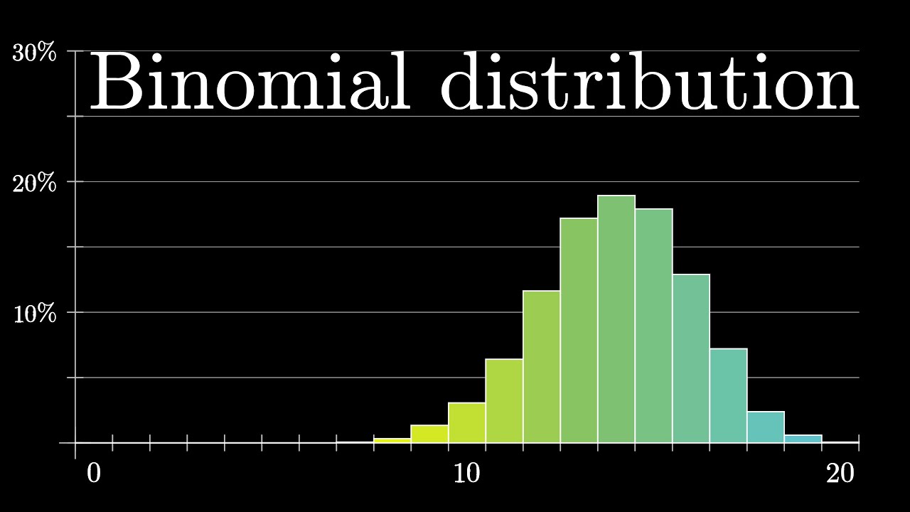
The Binomial Distribution
and start by talking about the binomial distribution. The second is going to bring in ideas of Bayesian updating, and how to work with probabilities over continuous values. And in the third, we'll look at something known as a beta distribution, and pull up a little python to analyze the data we have, and come to various different answers depending on what it is you want to optimize. Now, to throw you a bone before we dive into all the math, let me just show you what one of the answers turns out to be, since it's delightfully simple. When you see an online rating, something like this 10 out of 10, you pretend that there were two more reviews, one that was positive and one that's negative. In this case, that means you pretend that it's 11 out of 12, which would give 91. 7%. This number is your probability of having a good experience with that seller. So in the case of 50 reviews, where you have 48 positive and 2 negative, you pretend that it's 49 positive and 3 negative, which would give you 49 out of 52, or 94. 2%. That's your probability of having a good experience with the second seller. Playing the same game with our third seller who had 200 reviews, you get 187 out of 202, or 92. 6%. So according to this rule, it would mean your best bet is to go with seller number 2.
Laplace's Rule of Succession
This is something known as Laplace's rule of succession, it dates back to the 18th century, To understand what assumptions are underlying this, and how changing either those assumptions or your underlying goal can change the choice you make, we really do need to go through all the math. So without further ado, let's dive in. Step 1, how exactly are we modeling the situation, and what exactly is it that you want to optimize? One option is to think of each seller as producing random experiences that are either positive or negative, and that each seller has some kind of constant underlying probability of giving a good experience, what we're going to call the success rate
The Success Rate
or S for short. The whole challenge is that we don't know S. When you see that first rating of 100% with 10 reviews, that doesn't mean the underlying success rate is 100%. It could very well be something like 95%. And just to illustrate, let me run a little simulation, where I choose a random number between 0 and 1, and if it's less than 0. 95, I'll record it as a positive review, otherwise negative review. Now do this 10 times in a row, and then make 10 more, and so on, to get a sense of what sequences of 10 reviews for a seller with this success rate, would tend to look like. Quite a few of those, around 60% actually, give 10 out of 10. So the data we see seems perfectly plausible if the seller's true success rate was 95%. Or maybe it's really 90%, or 99%. The whole challenge is that we just don't know. As to the goal, let's say you simply want to maximize your probability of having a positive experience, despite not being sure of this success rate. So think about this here, we've got many different possible success rates for each seller, any number from 0 up to 1, and we need to say something about how likely each one of these success rates is, a kind of probability of probabilities. Unlike the more gamified examples like coin flips and die tosses and the sort of things you see in an intro probability class, where you go in assuming a long run frequency, like 1. 5 or 1. 6, what we have here is uncertainty about the long run frequency itself, which is a much more potent kind of doubt. I should also emphasize that this kind of setup is relevant to many situations in the real world where you need to make a judgment about a random process from limited data. For example, let's say that you're setting up a factory producing cars, and in an initial test of 100 cars, two of them come out with some kind of problem. If you plan to spin things up to produce a million cars, what are you willing to confidently say about how many total cars will have problems that need addressing? It's not like the test guarantees that the true error rate is 2%, but what exactly does it say? As your first challenge, let me ask you this. If you did magically know the true success rate for a given seller, say it was 95%, how would you compute the probability of seeing 10 positive reviews and 0 negative reviews, or 48 and 2, or 186 and 14? In other words, what's the probability of seeing the data given an assumed success rate? A moment ago I showed you something like this with a simulation, generating 10 random reviews, and with a little programming you could just do that many times, building up a histogram to get some sense of what this distribution looks like. Likewise, you could simulate sets of 50 reviews, and get some sense for how probable it would be to see 48 positive and 2 negative. You see, this is the nice thing about probability. A little programming can almost always let you cheat a little and see what the answer is ahead of time by simulating it. For example, after a few hundred thousand samples of 50 reviews, assuming the success rate is 95%, it looks like about 26. 1% of them would give us this 48 out of 50 review. Luckily, in this case, an exact formula is not bad at all. The probability of seeing exactly 48 out of 50 looks like this. This first term is pronounced 50 choose 48, and it represents the total number of ways that you could take 50 slots and fill out 48 of them. For example, maybe you start with 48 good reviews and end with 2 bad reviews, or maybe you start with 47 good reviews and then it goes bad good bad, and so on. In principle, if you were to enumerate every possible way of filling 48 out of 50 slots like this, the total number of these patterns is 50 choose 48, which in this case works out to be 1225. What do we multiply by this count? Well, it's the probability of any one of these patterns, which is the probability of a single positive review raised to the 48th times the probability of a single negative review squared. Crucial is that we assume each review is independent of the last, so we can multiply all the probabilities together like this, and with the numbers we have, when you evaluate it, it works out to be 0. 261, which matches what we just saw empirically with the simulation. You could also replace this 48 with some other value, and compute the probability of seeing any other number of positive reviews, again assuming a given success rate. What you're looking at right now, by the way, is known in the business as a
A Binomial Distribution
binomial distribution, one of the most fundamental distributions in probability. It comes up whenever you have something like a coin flip, a random event that can go one of two ways, and you repeat it some number of times, and what you want to know is the probability of getting various different totals. For our purposes, this formula gives us the probability of seeing the data given an assumed success rate, which ultimately we want to somehow use to make judgments about the opposite, the probability of a success rate given the fixed data we see. These are related, but definitely distinct. To get more in that direction, let's play around with this value of s and see what happens as we change it to different numbers between 0 and 1. The binomial distribution that it produces kind of looks like this pile that's centered around whatever s times 50 is. The value we care about, the probability of seeing 48 out of 50 reviews, is represented by this highlighted 48th bar. Let's draw a second plot on the bottom, representing how that value depends on s. When s is equal to 0. 96, that value is as high as it's ever going to get. And this should kind of make sense, because when you look at that review of 96%, it should be most likely if the true underlying success rate was 96%. As s increases, it kind of peters out, going to 0 as s approaches 1, since someone with a perfect success rate would never have those two negative reviews. Also, as you move to the left, it approaches 0 pretty quickly. By the time you get to s equals 0. 8, getting 48 out of 50 reviews by chance is exceedingly rare, it would happen 1 in 1000 times. This plot we have on the bottom is a great start to getting a more quantitative description for which values of s feel more or less plausible. Written down as a formula, what I want you to remember is that as a function of the success rate s, the curve looks like some constant times s to the number of positive reviews times 1 minus negative reviews. In principle, if we had more data, like 480 positive reviews and 20 negative reviews, the resulting plot would still be centered around 0. 96, but it would be smaller and more concentrated. A good exercise right now would be to see if you could explain why that's the case. There is a lingering question, though, of what to actually do with these curves. I mean, our goal is to compute the probability that you have a good experience with this seller, so what do you do? Naively, you might think that probability is 96%, since that's where the peak of the graph is, which in a sense is the most likely success rate. But think of the example with 10 out of 10 positives. In that case, the whole binomial formula simplifies to be s to the power 10. The probability of seeing 10 consecutive good reviews is the probability of seeing one of them raised to the 10th. The closer the true success rate is to 1, the higher the probability of seeing a 10 out of 10. Our plot on the bottom only ever increases as s approaches 1. But even if s equals 1 is the value that maximizes this probability, surely you wouldn't feel comfortable saying that you personally have a 100% probability of a good experience with this seller. Maybe you think that instead we should look for some kind of center of mass of this graph, and that would absolutely be on the right track. First, though, we need to explain how to take this expression for the probability of the data we're seeing given a value of s, and get the probability for the thing we actually don't know, given the data, know. And that requires us to talk about Bayes' rule, and also probability density functions. For those, I'll see you in part 2.