Backpropagation calculus | Deep Learning Chapter 4
10:17

Backpropagation calculus | Deep Learning Chapter 4

3Blue1Brown 03.11.2017 3 691 572 просмотров 74 355 лайков

Machine-readable: Markdown · JSON API · Site index

Поделиться Telegram VK Бот
Транскрипт Скачать .md
Анализ с AI
Описание видео
Help fund future projects: https://www.patreon.com/3blue1brown An equally valuable form of support is to share the videos. Special thanks to these supporters: http://3b1b.co/nn3-thanks Written/interactive form of this series: https://www.3blue1brown.com/topics/neural-networks 
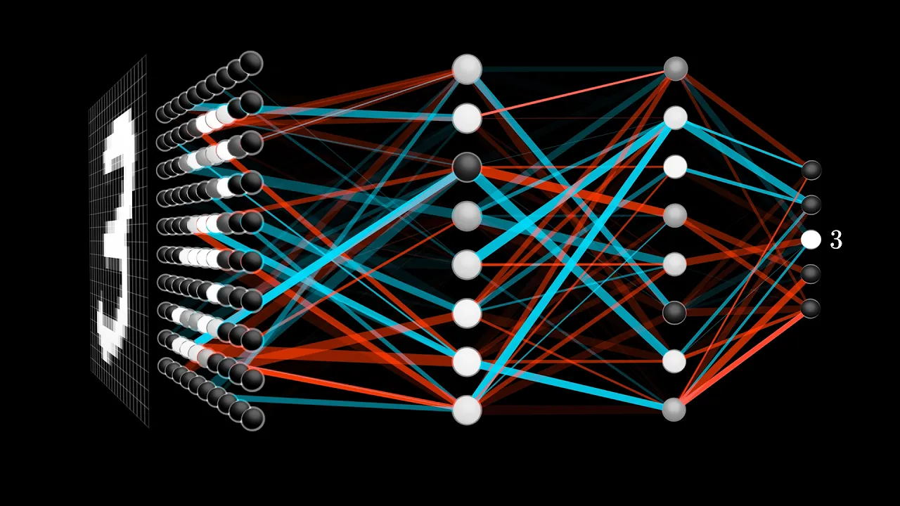
This one is a bit more symbol-heavy, and that's actually the point. The goal here is to represent in somewhat more formal terms the intuition for how backpropagation works in part 3 of the series, hopefully providing some connection between that video and other texts/code that you come across later. For more on backpropagation: http://neuralnetworksanddeeplearning.com/chap2.html https://github.com/mnielsen/neural-networks-and-deep-learning http://colah.github.io/posts/2015-08-Backprop/ Music by Vincent Rubinetti: https://vincerubinetti.bandcamp.com/album/the-music-of-3blue1brown Thanks to these viewers for their contributions to translations Звуковая дорожка на русском языке: Влад Бурмистров. Hebrew: Omer Tuchfeld ------------------ Video timeline 0:00 - Introduction 
0:38 - The Chain Rule in networks 3:56 - Computing relevant derivatives 4:45 - What do the derivatives mean? 5:39 - Sensitivity to weights/biases 6:42 - Layers with additional neurons 9:13 - Recap ------------------ 3blue1brown is a channel about animating math, in all senses of the word animate. And you know the drill with YouTube, if you want to stay posted on new videos, subscribe, and click the bell to receive notifications (if you're into that): http://3b1b.co/subscribe If you are new to this channel and want to see more, a good place to start is this playlist: http://3b1b.co/recommended Various social media stuffs: Website: https://www.3blue1brown.com Twitter: https://twitter.com/3Blue1Brown Patreon: https://patreon.com/3blue1brown Facebook: https://www.facebook.com/3blue1brown Reddit: https://www.reddit.com/r/3Blue1Brown

Оглавление (7 сегментов)

Introduction

[Submit subtitle corrections at criblate. com] The hard assumption here is that you've watched part 3, giving an intuitive walkthrough of the backpropagation algorithm. Here we get a little more formal and dive into the relevant calculus. It's normal for this to be at least a little confusing, so the mantra to regularly pause and ponder certainly applies as much here as anywhere else. Our main goal is to show how people in machine learning commonly think about the chain rule from calculus in the context of networks, which has a different feel from how most introductory calculus courses approach the subject. For those of you uncomfortable with the relevant calculus, I do have a whole series on the topic.

The Chain Rule in networks

Let's start off with an extremely simple network, one where each layer has a single neuron in it. This network is determined by three weights and three biases, and our goal is to understand how sensitive the cost function is to these variables. That way, we know which adjustments to those terms will cause the most efficient decrease to the cost function. And we're just going to focus on the connection between the last two neurons. Let's label the activation of that last neuron with a superscript L, indicating which layer it's in, so the activation of the previous neuron is a^(L-1). These are not exponents, they're just a way of indexing what we're talking about, since I want to save subscripts for different indices later on. Let's say that the value we want this last activation to be for a given training example is y, for example, y might be 0 or 1. So the cost of this network for a single training example is a^(L - y) squared. We'll denote the cost of that one training example as C0. As a reminder, this last activation is determined by a weight, which I'm going to call w(L), times the previous neuron's activation plus some bias, which I'll call b(L). And then you pump that through some special nonlinear function like the sigmoid or ReLU. It's actually going to make things easier for us if we give a special name to this weighted sum, like z, with the same superscript as the relevant activations. This is a lot of terms, and a way you might conceptualize it is that the weight, previous action and the bias all together are used to compute z, which in turn lets us compute a, which finally, along with a constant y, lets us compute the cost. And of course a(L-1) is influenced by its own weight and bias and such... but we're not going to focus on that right now. All of these are just numbers, right? And it can be nice to think of each one as having its own little number line. Our first goal is to understand how sensitive the cost function is to small changes in our weight w(L). Or phrased differently, what is the derivative of C with respect to w(L)? When you see this del w term, think of it as meaning some tiny nudge to W, like a change by 0. 01, and think of this del C term as meaning whatever the resulting nudge to the cost is. What we want is their ratio. Conceptually, this tiny nudge to w(L) causes some nudge to z(L), which in turn a(L), which directly influences the cost. So we break things up by first looking at the ratio of a tiny change to z(L) to this tiny change w(L), that is, the derivative of z(L) with respect to w(L). Likewise, you then consider the ratio of the change to a(L) to the tiny change in z(L) that caused it, as well as the ratio between the final nudge to C and this intermediate nudge to a(L). This right here is the chain rule, where multiplying together these three ratios gives us the sensitivity of C to small changes in w(L).

Computing relevant derivatives

So on screen right now, there's a lot of symbols, and take a moment to make sure it's clear what they all are, because now we're going to compute the relevant derivatives. The derivative of C with respect to a(L) works out to be 2(a(L)-y). Notice this means its size is proportional to the difference between the network's output and the thing we want it to be, so if that output was very different, even slight changes stand to have a big impact on the final cost function. The derivative of a(L) with respect to z(L) is just the derivative of our sigmoid function, or whatever nonlinearity you choose to use. And the derivative of z(L) with respect to w(L)... In this case comes out to be a(L-1).

What do the derivatives mean?

Now I don't know about you, but I think it's easy to get stuck head down in the formulas without taking a moment to sit back and remind yourself of what they all mean. In the case of this last derivative, the amount that the small nudge to the weight influenced the last layer depends on how strong the previous neuron is. Remember, this is where the neurons-that-fire-together-wire-together idea comes in. And all of this is the derivative with respect to w(L) only of the cost for a specific single training example. Since the full cost function involves averaging together all those costs across many different training examples, its derivative requires averaging this expression over all training examples. And of course, that is just one component of the gradient vector, which itself is built up from the partial derivatives of the cost function with respect to all those weights and biases.

Sensitivity to weights/biases

But even though that's just one of the many partial derivatives we need, it's more than 50% of the work. The sensitivity to the bias, for example, is almost identical. We just need to change out this del z del w term for a del z del b. And if you look at the relevant formula, that derivative comes out to be 1. Also, and this is where the idea of propagating backwards comes in, you can see how sensitive this cost function is to the activation of the previous layer. Namely, this initial derivative in the chain rule expression, the sensitivity of z to the previous activation, comes out to be the weight w(L). And again, even though we're not going to be able to directly influence that previous layer activation, it's helpful to keep track of, because now we can just keep iterating this same chain rule idea backwards to see how sensitive the cost function is to previous weights and previous biases.

Layers with additional neurons

And you might think this is an overly simple example, since all layers have one neuron, and things are going to get exponentially more complicated for a real network. But honestly, not that much changes when we give the layers multiple neurons, really it's just a few more indices to keep track of. Rather than the activation of a given layer simply being a(L), it's also going to have a subscript indicating which neuron of that layer it is. Let's use the letter k to index the layer L-1, and j L. For the cost, again we look at what the desired output is, but this time we add up the squares of the differences between these last layer activations and the desired output. That is, you take a sum over a(L)j minus yj squared. Since there's a lot more weights, each one has to have a couple more indices to keep track of where it is, so let's call the weight of the edge connecting this kth neuron to the jth neuron, w(L)_jk. Those indices might feel a little backwards at first, but it lines up with how you'd index the weight matrix I talked about in the part 1 video. Just as before, it's still nice to give a name to the relevant weighted sum, like z, so that the activation of the last layer is just your special function, like the sigmoid, applied to z. You can see what I mean, where all of these are essentially the same equations we had before in the one-neuron-per-layer case, it's just that it looks a little more complicated. And indeed, the chain-ruled derivative expression describing how sensitive the cost is to a specific weight looks essentially the same. I'll leave it to you to pause and think about each of those terms if you want. What does change here, though, is the derivative of the cost with respect to one of the activations in the layer L-1. In this case, the difference is that the neuron influences the cost function through multiple different paths. That is, on the one hand, it influences a(L)0, which plays a role in the cost function, but it also has an influence on a(L)1, which also plays a role in the cost function, and you have to add those up. And that, well, that's pretty much it. Once you know how sensitive the cost function is to the activations in this second-to-last layer, you can just repeat the process for all the weights and biases feeding into that layer.

Recap

So pat yourself on the back! If all of this makes sense, you have now looked deep into the heart of backpropagation, the workhorse behind how neural networks learn. These chain rule expressions give you the derivatives that determine each component in the gradient that helps minimize the cost of the network by repeatedly stepping downhill. If you sit back and think about all that, this is a lot of layers of complexity to wrap your mind around, so don't worry if it takes time for your mind to digest it all.

Методичка по этому видео

Структурированный конспект

Математика обратного распространения: исчисление за обучением нейросетей

Формальное объяснение математики обратного распространения ошибки (backpropagation) через цепное правило дифференцирования в контексте нейронных сетей.

Другие видео автора — 3Blue1Brown

Ctrl+V

Экстракт Знаний в Telegram

Экстракты и дистилляты из лучших YouTube-каналов — сразу после публикации.

Подписаться

Дайджест Экстрактов

Лучшие методички за неделю — каждый понедельник