Today on Applied Science, I'd like to show you this technique called compressed sensing. This allows us to reconstruct an image from just a tiny subset of pixels. It seems almost like magic that you could throw away 90% of an image's pixels and then reconstruct the image with surprisingly good fidelity. In fact, we can even reconstruct spatial frequencies that are higher than the so-called Nyquist limit, seemingly breaking the law of information theory. So in today's video I'm going to show you how this algorithm works and also how we can apply it to a real world device. This is a X-ray back scatter imaging system. And the reason that the algorithm is well suited to this piece of hardware is because acquiring each pixel takes us a long time. So we can't acquire every pixel in the image. We can only acquire a subset and then we use the algorithm to reconstruct the whole image. So, let's start off by talking about the X-ray back scatter itself. And then we'll talk about the algorithm. And in the next video, I'm going to show you how to apply this to the scanning electron microscope, another device that's limited by how long it takes to acquire each pixel in the image. X-ray back scatter imaging is really the closest thing we'll ever have to true X-ray goggles. You don't have to be behind the object. It's not like a shadow gram like most X-rays. And so the way this works is we shine a very thin beam of X-rays just like a laser pointer like this out into the scene and we collect the reflection the back scatter. So just like a laser pointer when you shine a beam of X-rays at something some of those X-rays are absorbed some are transmitted and some are reflected. And in the case of a laser pointer you'd say well you know light colored objects are more reflective than you know dark colored objects like this. And as it turns out with X-rays, the lower atomic number elements for a given density have more back scatter. So hydrogen, carbon, and oxygen are all very bright in these images. And higher atomic number elements are darker. And the really dense elements, high atomic number, high density elements are very dark because they absorb all the X-rays. The challenge is that this whole process is very lossy. To get high resolution, we have to have a tiny aperture here. This one is only 400 microns, which I found to work pretty well. So, we've got a 400 micron diameter beam of X-rays coming out to get good resolution, but that means there's a very, very small amount of X-rays hitting our object and then an even smaller a much smaller amount of reflection going back into our detector. So, at this point, we're really counting photons here. The detector has to be large area and it has to be super sensitive. And even then, we can't scan very quickly because we're just waiting for the photons to come in. So, the only way to make the system faster is to have a more intense X-ray beam or a bigger or more sensitive detector. And since we're already kind of counting photons here, we're not going to make it all that much more sensitive. So, really, it's just a bigger detector at that point. Or we can be clever and use this compressive sensing algorithm, which solves the problem very tidily. So to put some numbers on this, it takes us about 8 milliseconds to collect enough photons to get good dynamic range in our image. And so if we're scanning along, uh, if we want 1 millm resolution and we have a 60deree field of view, uh, let's say we want 800 by 800 pixels, just to make sure we're covered, even though that's sort of oversampling a little bit. If you pencil it all out, collecting the whole image, 800 by 800, 8 milliseconds per pixel, it comes out to something like 85 minutes to collect this whole X-ray back scatter image. And worse than that, if we really had to collect every pixel, the motion control system here would have to have incredibly good pointing accuracy. Um, it's one thing to measure the pointing accuracy. We can do that a lot easier than we can control it. And if we really have to collect every single pixel in the image, um, it's very difficult to just make sure there's no gaps anywhere. And, um, as I mentioned, measuring the position is relatively easy or easier than controlling it very precisely. So if this thing kind of jumps around a little bit or it's not a perfectly smooth or controlled sweep or this thing kind of jumps around a little bit, uh that's actually good with the compressive sensing algorithm as we'll see because it adds a little bit of randomness to how we're sampling the image. So instead of collecting every pixel, we're going to collect maybe one out of four pixels, which cuts our acquisition time down to just, you know, 10 or 20 minutes uh with comparable quality. I spent quite a bit of time trying to get the resolution as high as possible. Like I was willing to spend even more time per acquisition if I could get an even higher resolution image. But there's actually a limit here. I went down I tried different apertures from um you know 1. 2 mm 4 all the way down to 2 mm aperture to try to get the highest resolution possible. But I found that there's a limit that is I think based in materials and X-rays themselves that have nothing to do with the system. So imagine if you had a really ridiculously thin beam like a you know an infinitely fine beam going in there. What ends up happening is the X-rays
Segment 2 (05:00 - 10:00)
penetrate a little bit into the material and as the X-ray beam is going through you get back scatter from the depth of the material. So as we're scanning along you know there's going to be a loss of resolution. It might be, you might get one good edge here because as the beam sweeps along, the X-rays are missing the object, but as soon as it hits the object, you get all of this, you know, in just like the laser beam in this bottle of water, it kind of reflects around inside and you get a lot of back scatter from all depths of the image. So there is sort of a fundamental resolution limit that is not dependent on the hardware and trying to make this thing even higher resolution, which I wanted to do wasn't happening. So if anyone is really into this field, let me know if there actually is sort of a true limit to how much resolution you can get with X-ray back scatter imaging. Originally I had the idea of handholding the X-ray tube itself and just adding a gyroscope like an IMU to this. And this way you could measure the angular rotation um just randomly. Since this algorithm enjoys having random samples of the image, you could just handhold this thing and just swing it around anywhere. You wouldn't need it. this whole gimbal mount at all. You could literally just handhold the whole thing and just use the IMU to measure how it's moving through space. This actually does work. In fact, when I started this uh project, I was only using this gimbal to hold the tube and I was in fact moving it by hand through the whole range, not just one axis. Um, it does work. The problem is that you still have to collect, let's say, at the very least five minutes of data to get a decent looking image and ideally more like 10 or 20. And so that's just not happening. I mean, hold a hand holding this thing and swinging it around and inevitably you miss areas and so you need a UI to have feedback to show that you scanned through an area. Uh there still could be some applications if you really need a super low resolution image. Uh it does work. You can scan the whole thing yourself or potentially if you only scan one axis uh and you hand swing the other one basically that could also work quite well. Longtime viewers of the channel may recognize this. In fact, this is not my first X-ray back scatter imaging device. Uh, years ago, I used this same exact gimbal mount with a different X-ray tube and a spinning metal disc to basically cut the beam up and integrate the image using an oscilloscope, an analog oscilloscope screen with a long exposure camera shutter. I really can't believe I got away with this and made it work back in the day. As you can see, the image result is not, you know, the highest quality, but at the time, uh, the TSA was using these X-ray back scatter images to scan people getting on airplanes, and they have the ability to look through clothes, and it was a very controversial thing at the time because, you know, it shows you a very highly detailed image of someone's body through their clothes. Anyway, I think they got rid of all these X-ray back scatter imagers and um they're used now more for inspecting shipping containers and vehicles, looking for stuff that might be hidden in the vehicles. Let's talk about a few construction details. I'm using analog potentiometers to sense the rotation of both of these axes. Uh it's not the highest class solution, but it has the benefit of giving you absolute values. So, if the system power is cut, you know, you always get the same thing. And I'm using a Tinsi Arduino to coordinate this whole system. And all you have to do is say analog read and you get the position of that thing. You don't have to integrate anything or count anything. And it's also just physically easy to mount these. Um, for controlling the position, I have this DC gear motor and this weird little piece of latex that helps the gear teeth mesh here smoothly. Um, originally when I first thought of this system, I wasn't going to use motors. I was going to use my hand to move this around, but as it turns out, you know, it's just too slow. I just can't handhold it for that long. So, then I, you know, had the foresight of putting this little cog uh tooth belt uh pulley on the rotating part and I was going to use a 3D printed tooththed belt. This actually works really well. This is 3D printed TPU and you can just print any size cog belt you want. And I was going to use this to put it in here, but this is actually pretty stretchy and as it turns out, the inertia of this thing is very high. Okay. So, I needed a um a much tighter control loop. So, I just went with a direct gear connection there. And then similarly, there's just a 3D printed gear and a sector gear for the other axis. Also controlled by a DC gear motor. The two gear motors are controlled by these Hbridge motor drivers, L6203 motor drivers. And those are controlled by the Tinsy microcontroller. Here on the detector side, we've got this 3D printed black plastic structure. And inside there is a uh screen from an X-ray intensifier cassette. These are the things they used to use when doing film X-rays to expose the film more effectively. So instead of just using the X-rays to expose film directly, there's two sheets of phosphor in there that also produce light and expose the film more effectively. So I cut one of those sheets out and put it across in here and up and down the sides. And then
Segment 3 (10:00 - 15:00)
here we've got a photo multiplier tube, the high voltage supply for the photo multiplier. Uh here we've got a trans impedance amplifier to convert the current pulses from the photo multiplier into voltage spikes and then a coax to take the voltage spikes to the microcontroller. And conveniently the TNC 3. 2 has an analog comparator in hardware and a counter that you can connect the analog comparator to and output of the comparator to another physical pin here. So what this means is that we can count very low amplitude pulses even just 10 or 20 millolt pulses if they're that small and count them in a 16- bit counter without bothering or taking any CPU time at all. And uh you know eventually the counter overflows and you use an interrupt to sample that. But otherwise you don't um spend any CPU time. You can just query the register and get the count at any time. And it's convenient to see the output of the comparator so that we can debug this whole thing on the oscilloscope. Very convenient setup. The tiny also controls the X-ray tube over an RS232 serial link. And by an amazing stroke of luck, someone uploaded the programming manual to this X-ray tube to their GitHub, and I was able to figure out what the RS232 commands are. Um, I had to reverse engineer the pin out since this tube is not quite the same. But figuring out those um serial commands would have been a much more difficult challenge. If I didn't have the access to that, I would have had to isolate the two analog control voltages. Pretty much all these X-ray supplies work by having an analog control voltage for the high voltage like you know one volt scales up to 50,000 volts and then a control voltage for the current you know 1 volt scales up to 1 milliamp of current and this is a 50 kilovolt 1 milliamp X-ray tube. The tinsi constantly reports the position of the potentiometers and the number of counts that it got in the last 8 milliseconds from the photo multiplier and sends these over USB serial to the computer. And then I've got a processing. org script that just receives data over the serial port and plots them on the screen so we can see how it's doing and also saves it to a CSV file. And then we take the CSV file and send it over to another computer to be reconstructed in the algorithm. Quick note on X-ray safety. As I mentioned, the X-ray back scatter signal is so weak, we need a photon counter to even detect it at all. And so the thing you really have to worry about is the primary beam, which is directed down into the floor, the concrete floor of the shop. But just to be sure, I walked around the outside with my geer counter and of course cannot detect anything outside my shop, which I'm treating as the enclosure for this X-ray system. Let's talk about how this magic compressive sensing algorithm actually works. What we're going to do is reconstruct the image by just taking a bunch of points within it. But to make things easier to understand, we're going to look at this in just one dimension to start with. So let's say we're given a bunch of points and we're told that one frequency created this. Our job is to figure out what frequency fits best for these points for these measurements that we've taken. And we're told that the frequency is between 0 and 500 hertz. And we can use frequencies in one herz increments. It's pretty easy because we could just scale through all the frequencies. You know, try one herz, try two herz, try three. Eventually, we'll get one that fits pretty well and we can measure the fit after we've tried all of them. And there it is. That's the answer. Okay. Uh in the next setting of difficulty, we're given the points again. And this time we're told it's two frequencies mixed together. Uh so we try, you know, one hertz for frequency one and then scale through all the frequencies for frequency 2 and so on. And eventually we can come up with uh these two frequencies beated together again because we can try them all. Okay. Now we'll make it more difficult again. We're given all the points and this time we're told it could be any number of frequencies but our job is to basically reconstruct this using the fewest number of unique frequencies. Not the lowest frequencies but This is a much more challenging problem. even if we bound it by saying okay frequencies 0 to 500 in one herz increments um it's an optimization problem that has an infinite number of solutions. So for example we could get an okay fit with five frequencies but if we got an amazingly good fit with six frequencies which one do you pick? Well that's just a tuning parameter that we put into this algorithm. This is essentially what compressive sensing is doing. We're basically going to come up with a waveform that fits through all of these points using the minimal number of frequencies. And the last little bit of um trick that we're going to do here is if we sampled the frequency at the same interval over and over again like this, we wouldn't know if the true frequency is zero hertz or if it's, you know, one hertz like this high frequency like this. So, we can't
Segment 4 (15:00 - 20:00)
actually have regular sampling. What we want is to have completely random sampling in time. In fact, the more random the better because that allows us to figure out uh all of the frequency content where if we had regular sampling, we would have a blind spot where we couldn't pick apart certain things. But this is pretty mind-blowing. I mean, who's to say that if we use the fewest number of unique frequencies, we end up with the best representation of this image? Like, why is that even a law or a truth or anything? And this turns out to be a surprisingly deep question. So, think about it from an image standpoint. As it turns out, all of the natural images that you can find in the world, anything you can take with a camera, any X-ray back scatter image, any electron microscope image, even other types of signals, audio waveforms, you know, measurements of tides over time, any sort of a natural signal has this property that the number of unique frequencies making up that signal is minimized. This is sounds like a very sweeping generalization like how could this possibly be true? And so here's a funny way to think about it. Imagine you want a noise image. Like you go to image editing software and you generate noise or you turn on an analog television and tune to a station that's not there. Before you do this, you know what the image is going to look like, don't you? It looks like a bunch of black and white dots. It has a very characteristic pattern that you already anticipated when you asked for a noise image from this image editing software. Uh the interesting thing is how did you know what it was going to look like? Like really when you're asking for a noise image, what the software is doing is picking a random pixel and then going to the next pixel and picking another random value and then all the way down. So the chance that it generates a picture of a cat is actually exactly the same as the chance that it picks that exact noise image that it just showed you. But if the thing ever did generate a picture of a cat, you could file a bug and say, "Hey, your noise generator is broken. So the answer to why all noise images look like this. You know what a noise image looks like when you see one is because they are fundamentally different from any kind of a real image. And when I say a real image, it could be a photo taken with the lens cap on, out of focus, overexposed, it doesn't matter. It could be any kind of image that you created with a real device. And uh the reason for this is that there's just so many noise images. So think of it this way, right? If you generated that noise image and it's grayscale, the first pixel could be anywhere from 0 to 255 and then the next 255. So if you had a th00and by,000 pixel image, the total number of possible images is 255 to the 1 millionth power, which is far greater than the number of atoms in the universe or the number of plank times since the beginning of the universe. It's just an un an unbelievably large number. It's so large that when you generate a random image, it always ends up looking like noise because the probability that you're picking something in this huge space of images is so, you know, the chance that you would actually pick a cat or something that looks like a real thing is beyond low. It's actually basically impossible. And so all of the real images in the world share this property that they don't have uncorrelated stuff going on between all the pixels. And so the way this algorithm works is it minimizes the chance that it reconstructs a noise image which you know occupies the vast majority of possible images and maximizes the chance that it reconstructs a real image which is this tiny sliver of all the possible images. Now it may still seem a little unsatisfying that natural images this tiny sliver of all possible images uh share the property that they minimize the number of spatial frequencies that make them up. I don't know if there's a better sort of explanation for why that's the case. It's just one of these universal laws that is pretty interesting. It's not something that humans created. It's just a universal thing. Um, but of course, if you're interested in this, there's hour-long lectures on YouTube that I'll link to that go into the mathematical rigor. Obviously, this is a whole field of study, and I'm not a mathematician or an information theorist. And if you're interested in this, I encourage you to look into it even more. I know what some of you are thinking. What if I went to the beach and took a picture of the sand and set it up so that each grain of sand was one pixel in my image? Clearly, that would be random. Yes, I think it would. Uh there's always interesting edge cases and I think that is probably one of them. Another thing to keep in mind is it's not like the system works and then you'll find an edge case and it's broken. It's kind of like a sliding scale. So we could take images that challenge the algorithm and don't really follow this property very well like a picture of sand and you can go all the way to a true noise image that this algorithm could never reconstruct because that's not what it's looking for. So it's always good to keep in mind that uh nothing is perfect and even images that it's recreating are not perfectly recreated because you know the algorithm doesn't know what data was there. So all it can do is follow this
Segment 5 (20:00 - 20:00)
law and everything is a little bit non ideal. But anyway, like I say, most of my videos are designed to get your interest up in a topic and just show you something interesting and encourage you to do some more research on YouTube that I'll help you link to. Um, all the stuff I talked about in the video today will be up on GitHub. And uh, I hope you found it interesting and I will see you next time. Bye.